dataviz
Health Uyari
- License — License: MIT
- Description — Repository has a description
- Active repo — Last push 0 days ago
- Low visibility — Only 9 GitHub stars
Code Gecti
- Code scan — Scanned 12 files during light audit, no dangerous patterns found
Permissions Gecti
- Permissions — No dangerous permissions requested
Bu listing icin henuz AI raporu yok.
Fast pure-Rust plotting: 120+ chart types incl. 3D (molecules, DNA, isosurfaces), genomics, trading and ML charts, live windows, animations, maps, HTML/PNG/SVG/PDF, WebAssembly, and a Claude Code plugin. Faster and lighter than plotters.
DataViz 🚀


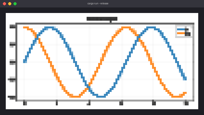
Fast, pure-Rust plotting: 120+ chart types, interactive windows, live
data, animations, maps, math and every language — with the least CPU and
memory of the Rust plotting libraries.
 |
 |
 |
 |
 |
 |
Why dataviz
- Fast and lean. Its own rasterizer draws straight into the output
buffer: a 10-million-point line renders in about 0.1 s with a few MB of
extra memory, a live chart redraws in 1–2 ms. 8–50× faster than
matplotlib, and faster and lighter than plotters, ruviz, kuva and
charts-rs in nearly every measurement (numbers below).
Optional multi-core and GPU backends. - Everything in one crate. 120+ chart types — lines, bars, statistics,
heatmaps, contours, 3D, maps, sankey, networks — plus ready-made charts
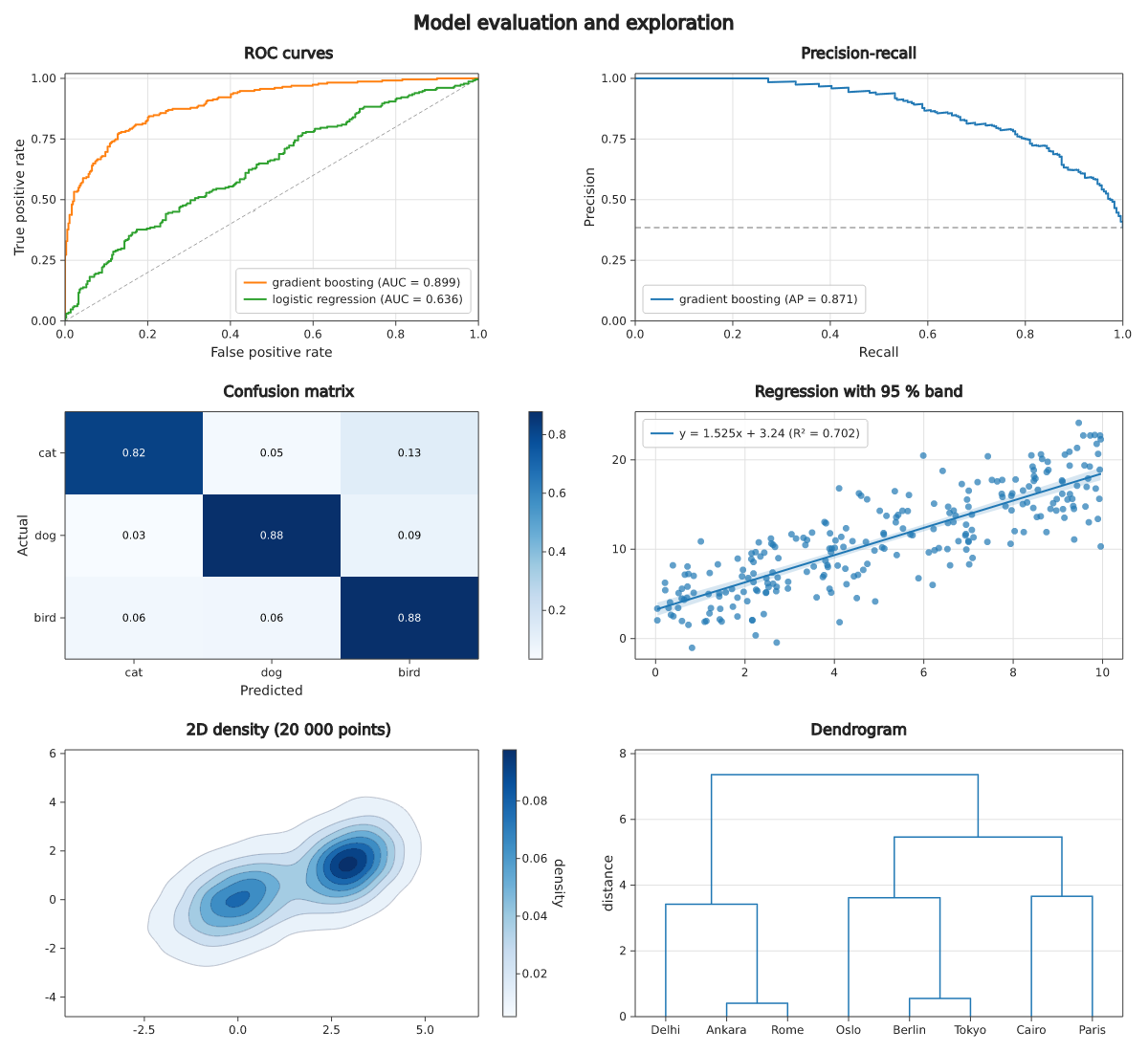
for data scientists (ROC/PR curves, confusion matrices, regression
bands, density contours, dendrograms), biologists and clinicians
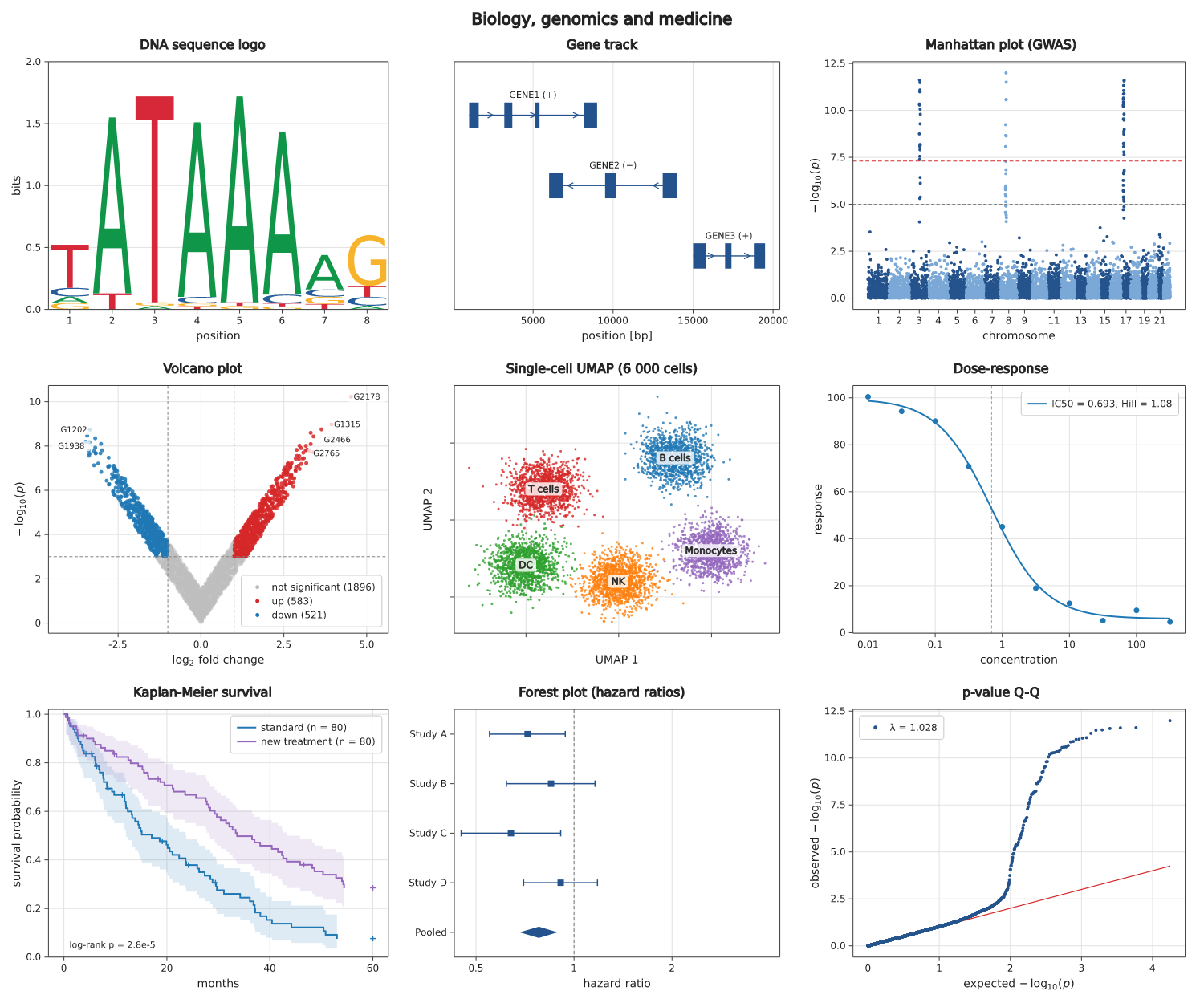
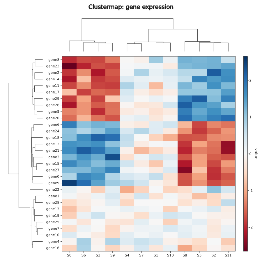
(DNA sequence logos, gene tracks, Manhattan, volcano, clustermaps,
single-cell UMAPs, dose-response, Kaplan-Meier, forest plots),
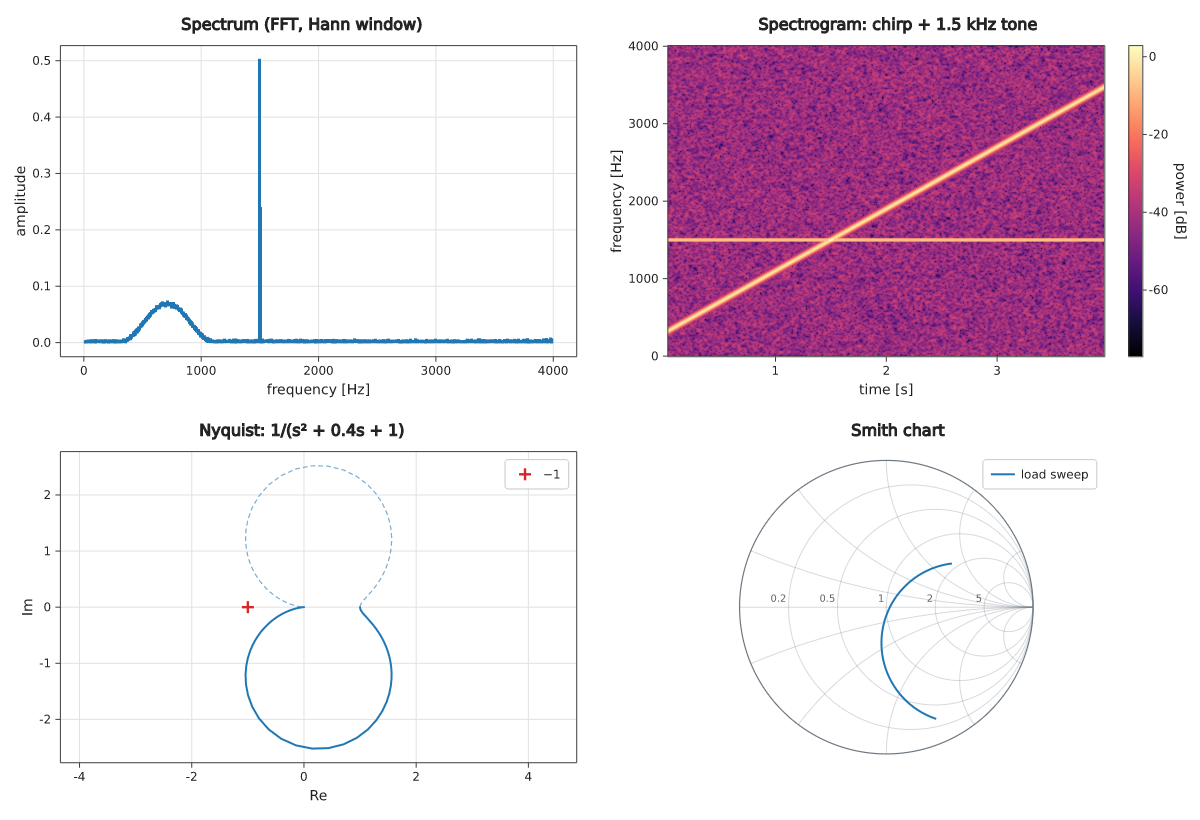
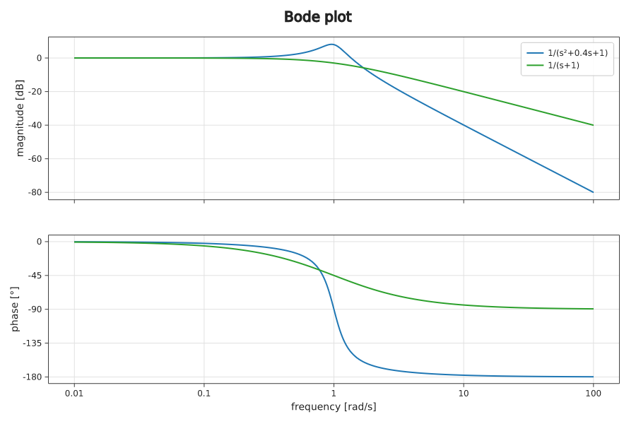
engineers (FFT spectra, spectrograms, Bode, Nyquist, Smith charts)
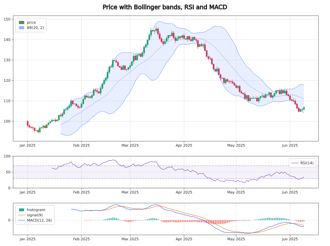
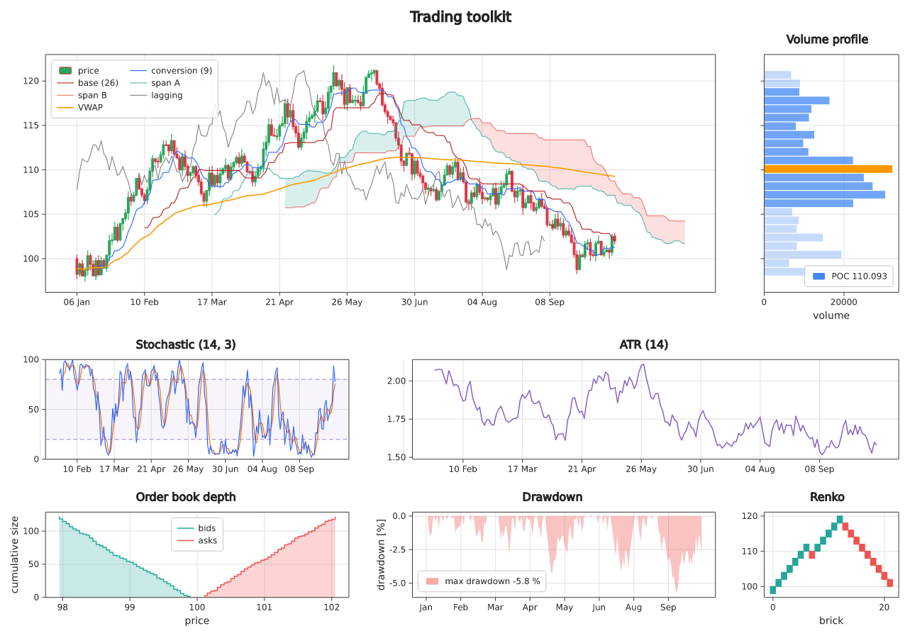
and traders (candlesticks,
Ichimoku, VWAP, RSI, MACD, volume profile, order book depth, drawdown,
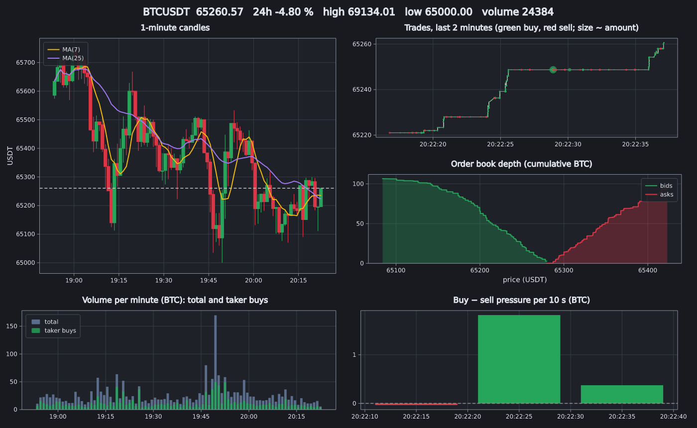
Renko), with themes, subplots, shared and broken axes. - Interactive and live.
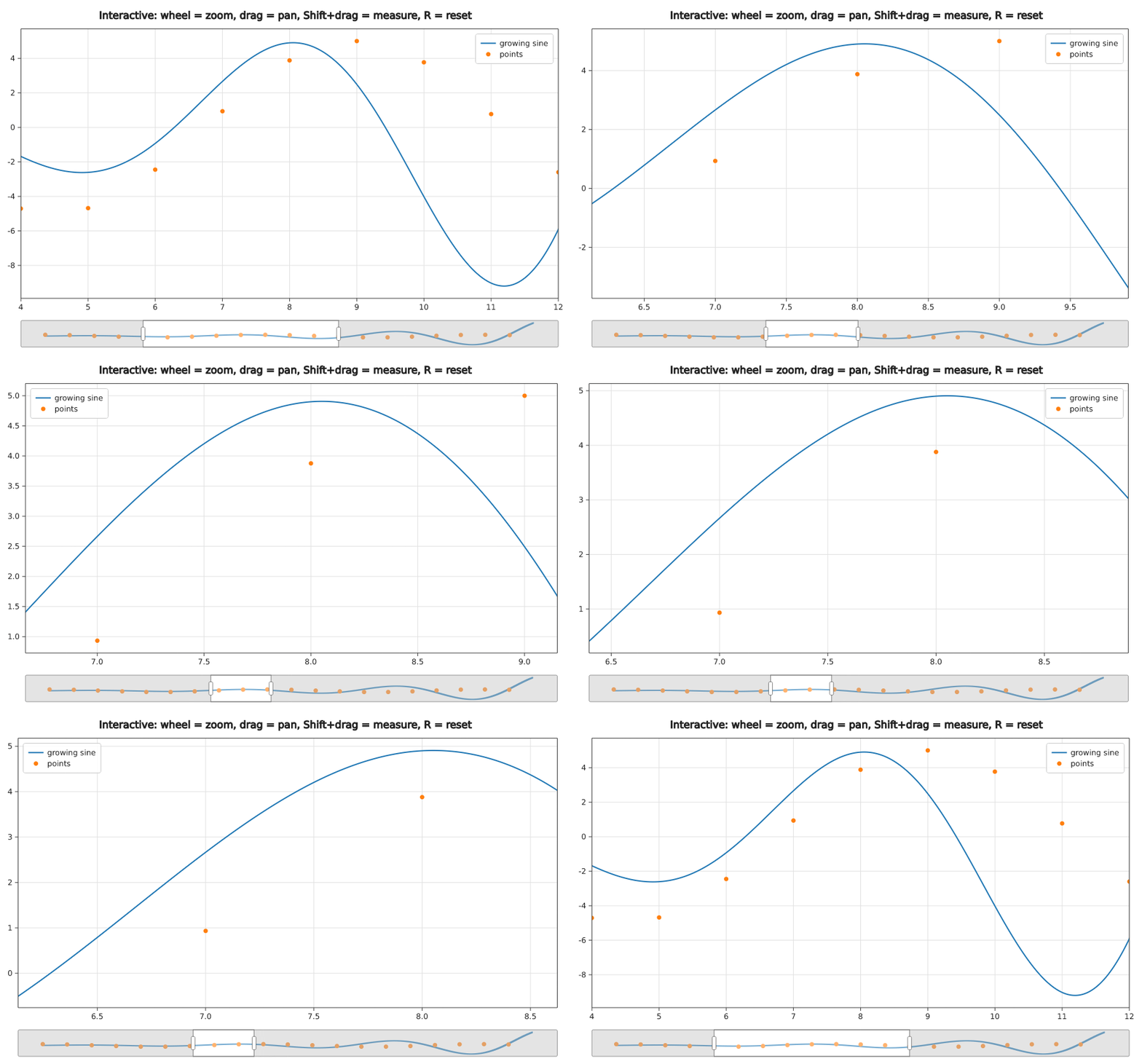
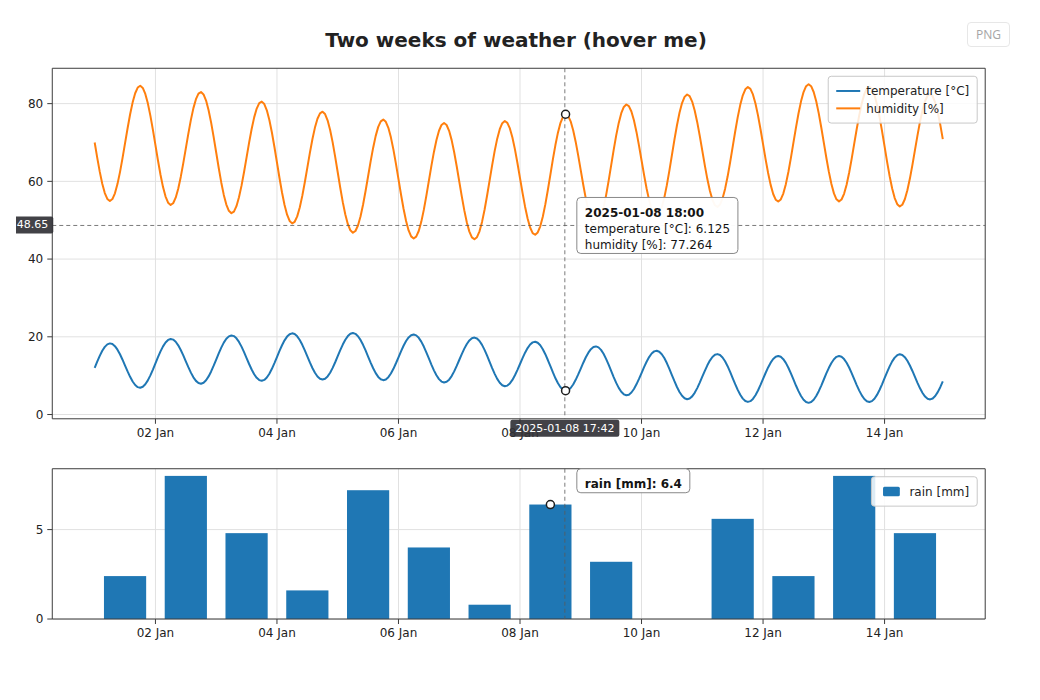
fig.show()opens a window with zoom, pan, a
crosshair with axis values, hover readouts, legend toggling, a range
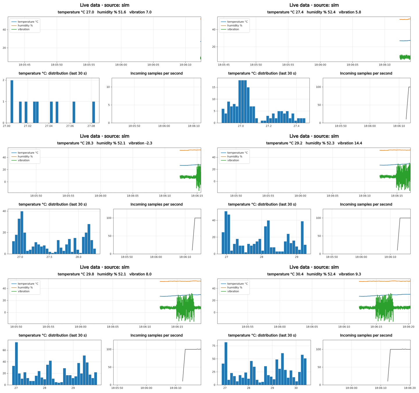
slider, measurement and selection;fig.show_live()streams data with
rolling windows and records it to CSV or a GIF. - Every output. PNG, SVG, PDF, JPEG, WebP, interactive HTML (one file,
no internet needed), animated GIF/PNG and MP4, the terminal, raw pixels
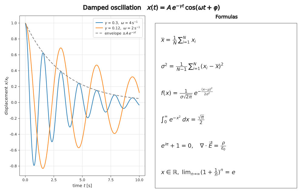
for your own GUI, and the browser via WebAssembly. - Text done right. TeX math (
$\sigma^2 = \frac{1}{N}\sum x_i^2$) in
every label, any language (CJK, Arabic and Hebrew right to left, Hindi,
Thai) and color emoji. - Accessible. Generated text descriptions for screen readers, color
blindness simulation and warnings for colors that look alike. - Pure Rust, few dependencies. No Python, JavaScript, browser,
Cairo or system fonts needed (a font is embedded); builds headless and
forwasm32.
Quick start
[dependencies]
dataviz = "0.15"
use dataviz::prelude::*;

fn main() -> Result<(), Error> {
    let x: Vec<f64> = (0..200).map(|i| i as f64 / 20.0).collect();

    let mut fig = Figure::new(900, 500);
    let ax = fig.axes();
    ax.title("Signals").x_label("time [s]").y_label("amplitude");
    ax.line(&x, x.iter().map(|t| t.sin())).label("sin");
    ax.line(&x, x.iter().map(|t| t.cos())).label("cos").dash(Dash::Dashed);
    ax.scatter([1.6, 4.7, 7.9], [1.0, -1.0, 1.0]).label("peaks").marker(Marker::Star).size(12.0);

    fig.save("signals.png")?;   // .svg .pdf .html .jpg .webp .bmp
    fig.show("Signals")?;       // interactive window
    Ok(())
}
Every chart type has a runnable example with code and output in
dataviz-examples — see
the gallery.
Your data, as it is
Any iterable of numbers works — Vec, slices, ranges, iterators and arrays
from other crates, without conversion or features:
ax.line(&x, &y); // Vec<f64>, &[f32], i64, …
ax.line(&array1, &array1.mapv(f64::sin)); // ndarray
ax.line(×, polars_df.column("price")?.f64()?); // Polars (nulls become gaps)
ax.scatter(arrow_x.values(), &arrow_y); // Arrow Float64Array
let t = dataviz::plot::data::Table::read("data.csv")?; // CSV/TSV, quoted fields
ax.line(t.time_column("date").unwrap(), t.column("close").unwrap());
Features
Interactive windows and live data
fig.show("title")?;                          // static data
fig.show_live("title", 30, |fig| { /* push new points */ true })?;
| Mouse / key | Action |
|---|---|
| wheel, drag, right-drag | zoom around the cursor, pan, zoom to a box |
crosshair (C) |
cursor values on the axes and every series' value at that x; linked across plots sharing x |
hover (H) |
nearest data point |
| click a legend row | hide or show the series |
| range slider | drag to pan, drag its edges to zoom |
| Shift+drag / Ctrl+drag | measure Δx, Δy and % / select a box (fig.selection()) |
A, R |
auto scale y to the visible data, follow live data again |
S, Shift+S, Ctrl+C, V |
save PNG, SVG/PDF, copy to the clipboard, record a GIF |
3D: drag, wheel, X/Y/Z |
turn the scene, zoom, rotate 15° around that axis (Shift = reverse) |
Live charts keep the view you zoomed to while data arrives (y follows the
visible data), stream with Line::push / keep_last / keep_since, andplot::data::CsvLog records the stream to CSV. The same zoom, pan, hover
and click work in your own GUI or web page throughfig.zoom_at, pan_by, hover, click (egui,
WebAssembly).
Chart types
| Category | Charts |
|---|---|
| Lines & areas | line, step, smooth spline, area, fill-between, stacked / 100 % area, streamgraph, horizon chart, function plot, sparkline |
| Points | scatter, colormapped scatter, bubble |
| Bars | vertical, horizontal, grouped, stacked, percent, overlay, value labels, waterfall, Gantt, lollipop, bullet, dumbbell, Pareto |
| Distributions | histogram (bin rules, density, cumulative, step), KDE, ECDF, box (notches), violin, raincloud, strip, swarm, ridgeline, Q-Q, 2D histogram, hexbin |
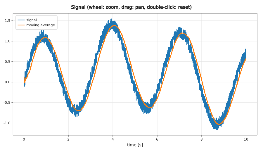
| Uncertainty & fits | error bars, error bands, polynomial regression with R², moving averages |
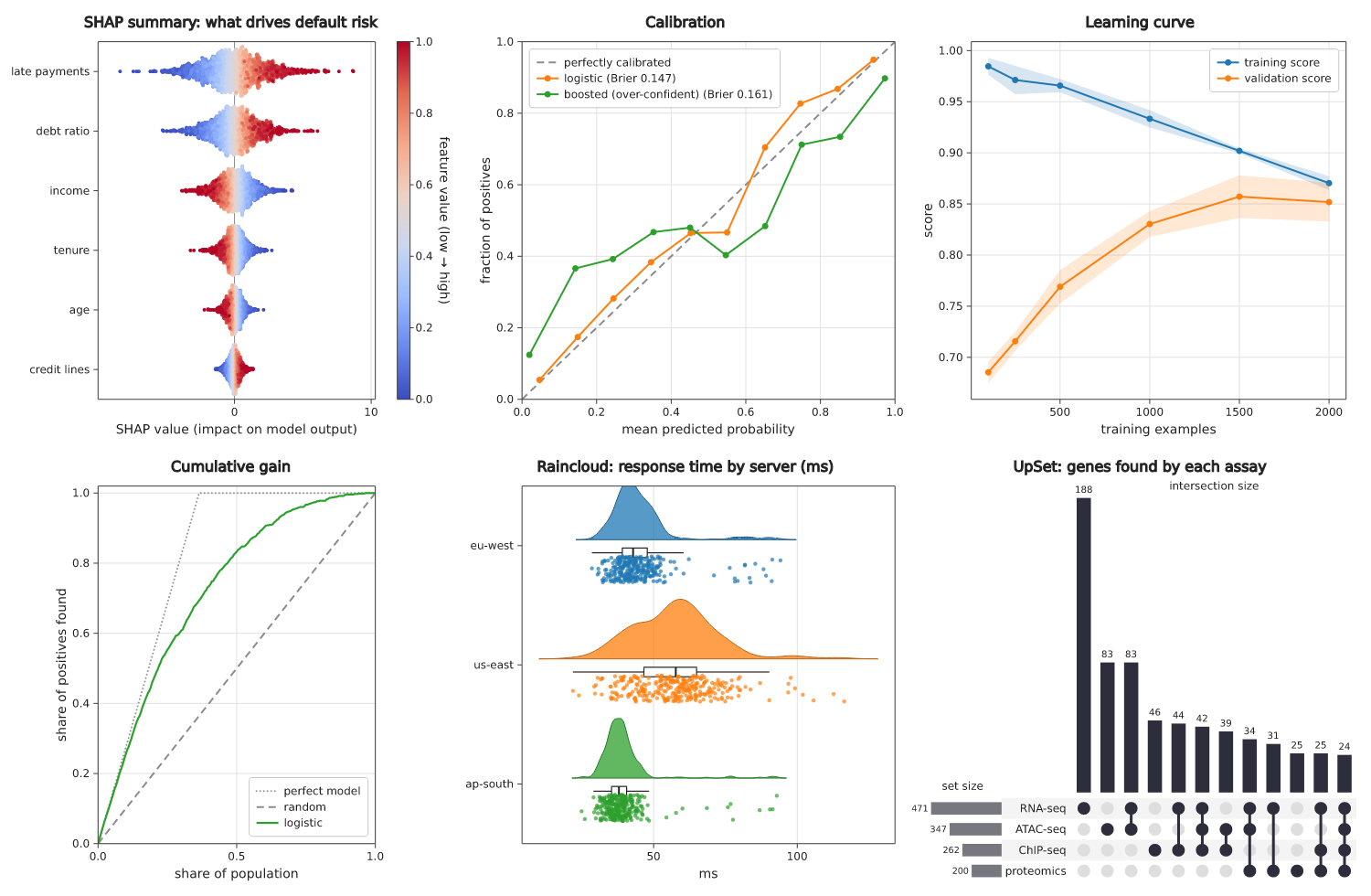
| Machine learning | ROC curve (AUC), precision-recall curve, confusion matrix, SHAP summary, calibration curve, learning curve, cumulative gain and lift, regression with confidence band, LOESS, 2D density contours, dendrogram, UpSet plot |
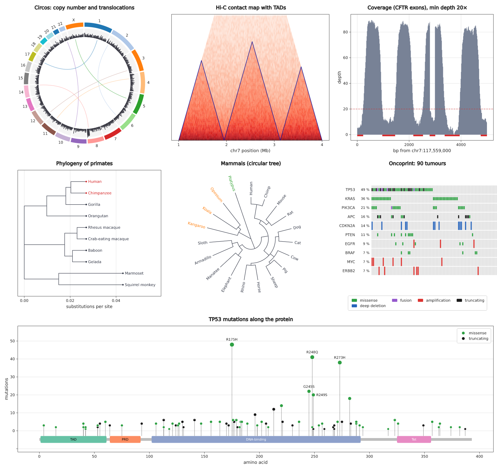
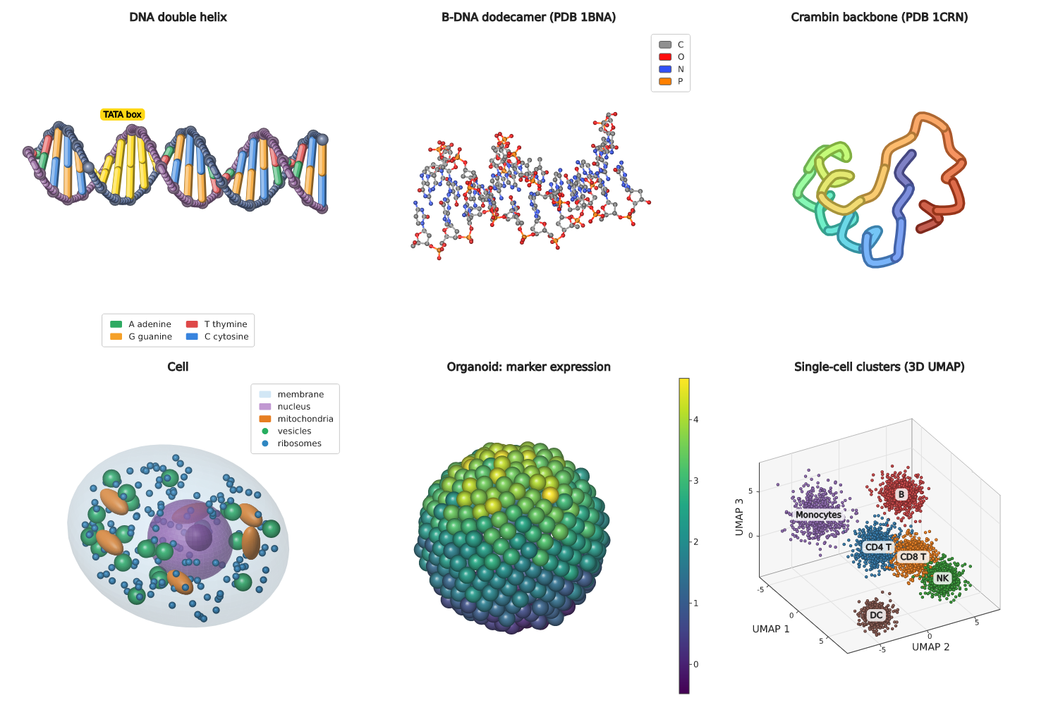
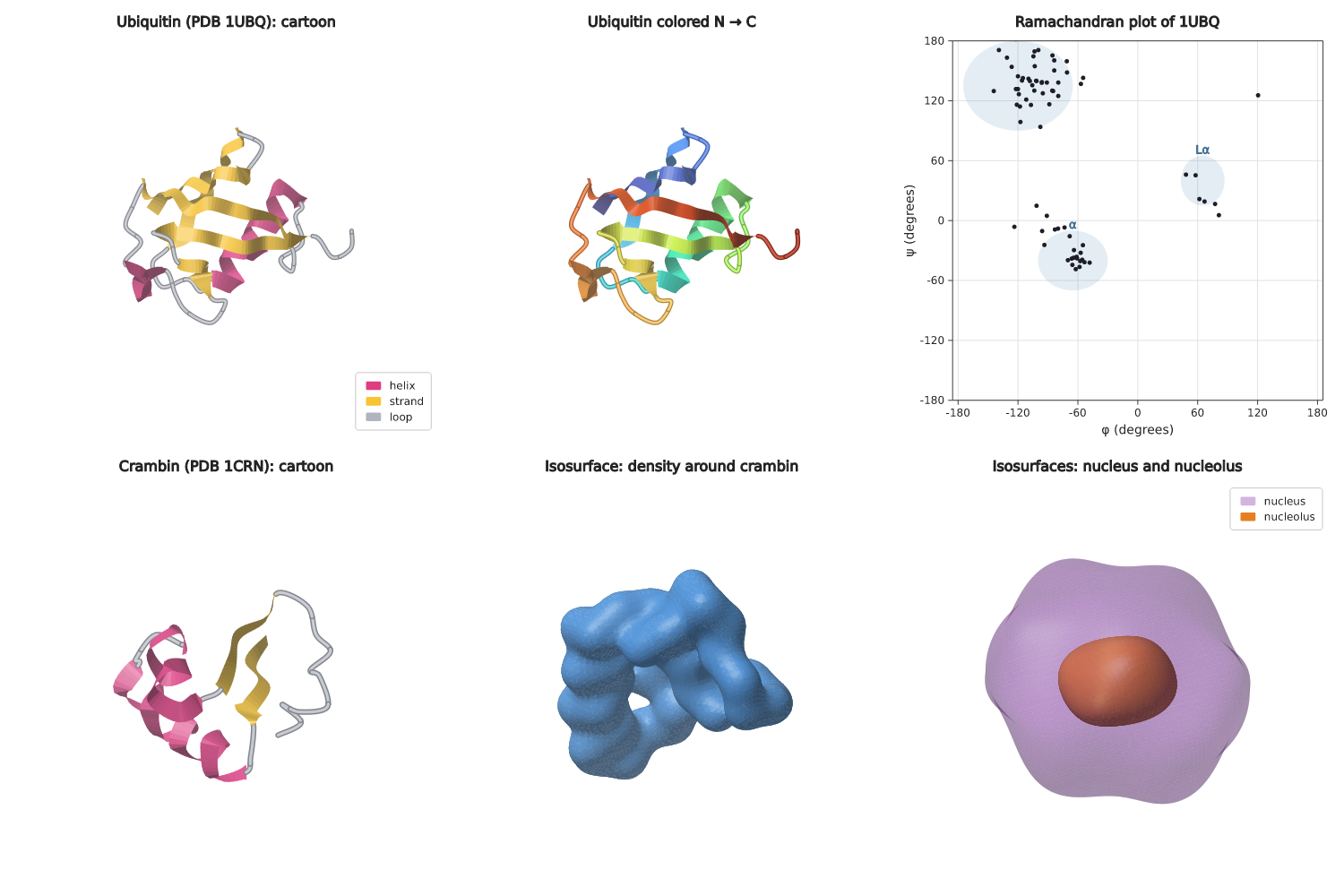
| Biology & medicine | 3D DNA double helix, molecules from PDB/XYZ (ball-and-stick, sticks, space-filling, backbone, cartoon), Ramachandran plot, isosurfaces of volumes, 3D cells and organoids, 3D UMAP, Circos, Hi-C contact map, coverage track, phylogenetic trees (Newick; rectangular, circular), oncoprint, mutation lollipop, DNA/protein sequence logo, gene track, Manhattan plot, p-value Q-Q, volcano plot, MA plot, clustermap, single-cell embedding (UMAP/t-SNE), dose-response (IC50), Kaplan-Meier survival, forest plot |
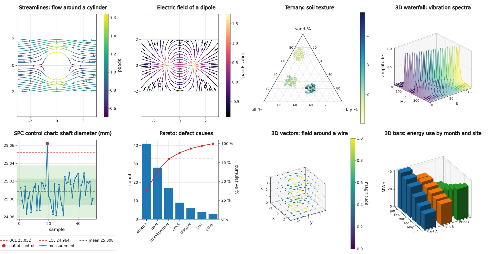
| Signals & control | FFT spectrum, spectrogram, 3D waterfall, Bode plot, Nyquist plot, Smith chart, streamlines, SPC control chart |
| Finance & trading | candlestick, OHLC, Heikin-Ashi, Renko, footprint (order flow), market profile (TPO), liquidity heatmap, option payoff (Black–Scholes), implied volatility surface, Bollinger bands, Ichimoku cloud, VWAP, RSI, MACD, Stochastic, ATR, volume profile, order book depth, drawdown, trading-day axis |
| Grids & fields | heatmap, correlation matrix, calendar heatmap, image, contour lines and fills, quiver |
| 3D | surface, wireframe, scatter, line, spheres, meshes, ellipsoids, isosurfaces, vectors, bars, text; one shared scene per plot with depth sorting, lighting, perspective and free rotation around x, y and z |
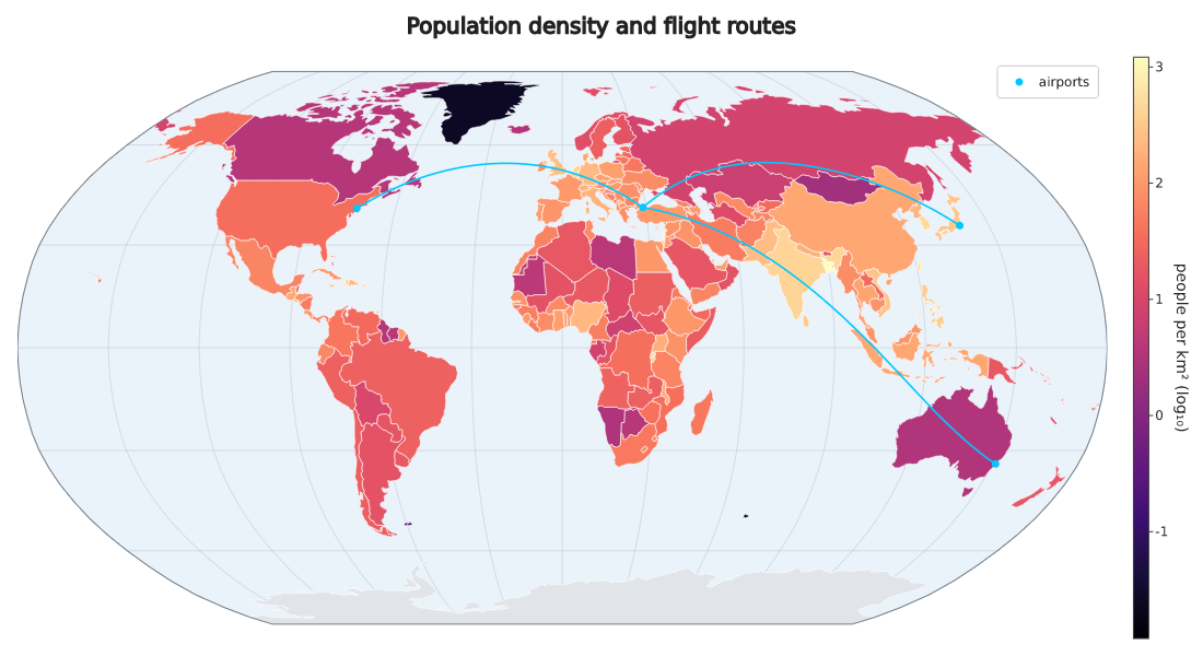
| Maps | built-in world map, choropleth by ISO code or name, points and great-circle routes, GeoJSON shapes; Robinson, Natural Earth, equirectangular, Mercator |
| Parts of a whole | pie, donut, treemap, sunburst, waffle, marimekko (mosaic), funnel, gauge |
| Polar | polar line/scatter, radar, rose / wind rose |
| Relations & flows | sankey, chord diagram, network graph (force-directed), parallel coordinates, slope chart, bump chart, ternary diagram |
| Layouts | subplots with spans, shared axes, broken axes, secondary y-axis, facets (small multiples), pair plot, aligned panels |
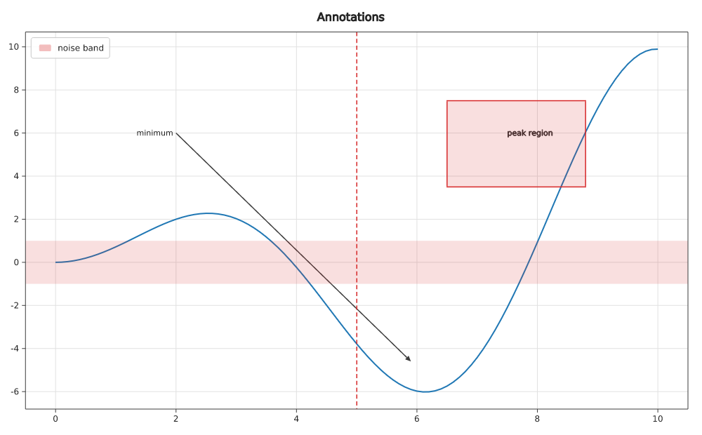
| Annotations | text, arrows, reference lines, shaded spans, rectangles |
For data scientists
ax.roc_curve("gradient boosting", &labels, &scores);    // legend shows the AUC
ax.pr_curve("gradient boosting", &labels, &scores);     // and the average precision
ax.confusion_matrix(["cat", "dog", "bird"], &actual, &predicted, true);
ax.regplot(&x, &y);                                     // fit, 95 % band and R²
ax.density_contour(&x, &y);                             // 2D KDE, millions of points
ax.dendrogram(&names, &features);                       // hierarchical clustering
ax.shap_summary(&features, &shap, &values, 10);         // what drives the model
ax.calibration_curve("model", &labels, &probs, 10);     // Brier score in the legend
ax.learning_curve(&sizes, &train, &validation);
ax.gain_curve("model", &labels, &scores);               // and lift_curve
ax.raincloud([("A", &a), ("B", &b)]);
ax.upset(&sets, 12);                                    // set intersections
For biologists and clinicians
ax.sequence_logo(&aligned_sequences);                   // DNA, RNA or protein motif
ax.gene_track(&genes);                                  // exons, introns, strand
ax.manhattan(&chromosome, &position, &p_values);        // GWAS
ax.volcano(&genes, &log2_fc, &p_values, 1.0, 1e-3, 10); // top 10 genes named
fig.clustermap(&genes, &samples, &expression);          // clustered heatmap
ax.embedding(&umap_x, &umap_y, &cell_types);            // single-cell clusters
ax.dose_response(&concentration, &viability);           // 4PL fit and IC50
ax.kaplan_meier([("control", t1, e1), ("treated", t2, e2)]); // log-rank p
ax.forest_plot(&studies, &hr, &low, &high, 1.0);        // meta-analysis
ax.circos(&chromosomes).track(&chr, &pos, &cn).links(&sv);
ax.hic(matrix, start, bin).domains(&tads);              // contact map as a triangle
ax.coverage(&pos, &depth).min_depth(20.0);
ax.phylo_tree(newick);                                  // or phylo_tree_circular
ax.oncoprint(&genes, samples, &alterations);
ax.mutation_lollipop(393.0, &domains, &mutations);
ax.molecule(Molecule::from_pdb(&pdb)).style(MolStyle::Cartoon);
ax.ramachandran(&phi, &psi);                            // from molecule.phi_psi()
ax.isosurface(&volume, [nx, ny, nz], bounds, level);    // microscopy, CT, densities
3D: rotate around x, y and z
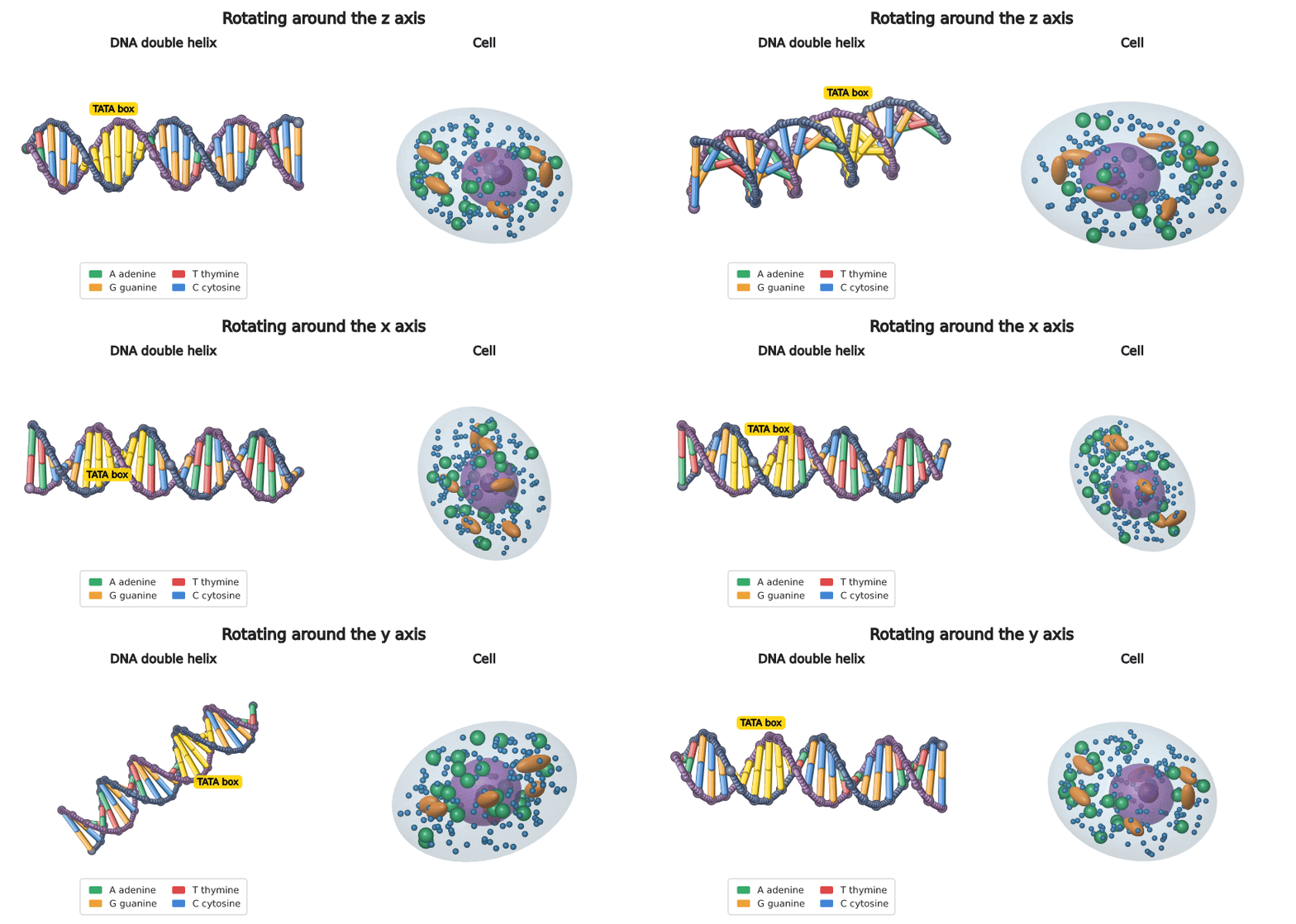
ax.dna_helix("ATGCGTATAAAAGCC").highlight(5..11, "#ffd400", Some("TATA box"));
ax.molecule(Molecule::from_pdb(&pdb)).style(MolStyle::Backbone).coloring(MolColor::Rainbow);
ax.ellipsoid([0.0, 0.0, 0.0], [10.0, 8.0, 6.0]).opacity(0.16);   // a cell membrane
ax.spheres3d(&x, &y, &z, [1.0]).values(&expression, Colormap::Viridis);
ax.embedding3d(&umap1, &umap2, &umap3, &cell_types);
ax.surface_fn(|x, y| (x * y).sin(), (-3.0, 3.0), (-3.0, 3.0), 60);
ax.rotate(Axis3::X, 30.0).roll(10.0).perspective(0.4);       // or ax.camera(azimuth, elevation)
All 3D series of a plot share one scene, sorted by depth, lit from the
upper left and optionally faded with distance (depth_cue). The camera is
a rotation matrix, so it turns freely around any axis. In a window: drag
to turn, wheel to zoom, X/Y/Z rotate by 15° (Shift+key the other
way), R resets, hover names the atom, base pair or point. A frame of the
1BNA DNA structure (486 atoms, ball-and-stick, shaded) takes about 8 ms on
one core, a 10 000-point 3D scatter 3 ms; a turning 90-frame GIF of a
surface 0.9 s (3D benchmarks in the Performance section).
For engineers
use dataviz::plot::series::signal::{freq_response, logspace};
ax.spectrum(&signal, 8000.0);                           // FFT amplitude spectrum
ax.spectrogram(&signal, 8000.0, 512, 64);               // STFT power in dB
let w = logspace(0.01, 100.0, 400);
fig.bode("plant", &w, &freq_response(&[1.0], &[1.0, 0.4, 1.0], &w));
ax.nyquist(&freq_response(&[1.0], &[1.0, 0.4, 1.0], &w));
ax.smith(&impedances);                                  // normalized z on a Smith chart
ax.streamplot(|x, y| (u(x, y), v(x, y)), (-3.0, 3.0), (-2.0, 2.0), 28);
ax.ternary(&a, &b, &c).names("sand", "silt", "clay");
ax.waterfall3d(&freq, &time, spectra);
ax.control_chart(&measurements);                        // ±3σ, Western Electric rules
ax.pareto(&causes, &counts);
ax.quiver3d(points, vectors);
For traders
let x = ax.trading_axis(×, "%d %b"); // no weekend gaps
ax.candlestick(&x, &open, &high, &low, &close);
ax.ichimoku(&x, &high, &low, &close);
ax.vwap(&x, &high, &low, &close, &volume);
profile.volume_profile(&close, &volume, 24); // POC and value area
osc.stochastic(&x, &high, &low, &close, 14, 3);
book.depth_chart(&bids, &asks);
dd.drawdown(&x, &equity); // max drawdown in the legend
heat.liquidity_heatmap((t0, t1), (p0, p1), &depth); // order book over time
of.footprint(bars, 0.25); // bid × ask per level
tpo.market_profile(&ranges, 1.0); // POC and value area
opt.option_payoff(&legs, (80.0, 120.0), 30.0, 0.22, 0.03);
vol.volatility_surface(&strikes, &maturities, &iv);
Business and editorial
ax.bullet(&kpis, &values, &targets, &ranges);
ax.dumbbell(&names, &before, &after);
ax.slope(&names, &before, &after, "2020", "2025");
ax.bump(&teams, &seasons, &ranks);
ax.waffle(&parts, &shares);
ax.marimekko(&columns, &rows, &values);
ax.chord(&groups, &flows);
ax.streamgraph(&x, &layers);
ax.horizon(&x, &rows);
Statistics and finance
ax.violin([("A", &a), ("B", &b)]);
ax.swarm([("A", &a), ("B", &b)]);
ax.ridgeline(months);                      // (name, values) per row
ax.qq(&values);                            // against the normal distribution
ax.regression(&x, &y, 2);                  // label shows the equation and R²
fig.facet_wrap(groups, 3, |ax, data| { ax.line(&t, data); });
fig.pair_plot([("length", &l), ("weight", &w), ("age", &a)]);

ax.candlestick(&t, &open, &high, &low, &close);
ax.bollinger(&t, &close, 20, 2.0);
rsi_panel.rsi(&t, &close, 14);
macd_panel.macd(&t, &close, 12, 26, 9);
Maps
use dataviz::plot::geo::Projection;
ax.map(Projection::Robinson);
ax.choropleth([("DEU", 83.2), ("TUR", 85.3), ("JP", 124.5), ("Brazil", 203.1)])
    .colorbar("population [M]");
ax.geo_line([28.98, -74.0], [41.01, 40.7]);    // great circle Istanbul → New York
Country outlines with ISO codes, continent, population and GDP are
included (Natural Earth, public domain); geo::read_geojson reads other
shapes.
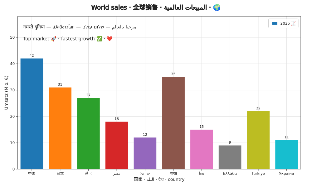
Text: math and any language
ax.y_label(r"$\sigma^2$ [$\mathrm{m^2\,s^{-2}}$]");
ax.text(1.0, 2.0, r"$\int_0^\infty e^{-x^2}\,dx = \frac{\sqrt{\pi}}{2}$");
fig.title("Ventes · 全球销售 · المبيعات · 🚀");
TeX math (scripts, fractions, roots, Greek letters, operators, accents) is
typeset in PNG, SVG, PDF and on the GPU alike. Characters missing from the
embedded font come from system fonts; right-to-left text is reordered and
shaped; color emoji are drawn.
Output
fig.save("chart.png")?;            // also .svg .pdf .jpg .webp .bmp
fig.save("chart.html")?;           // interactive, self-contained page
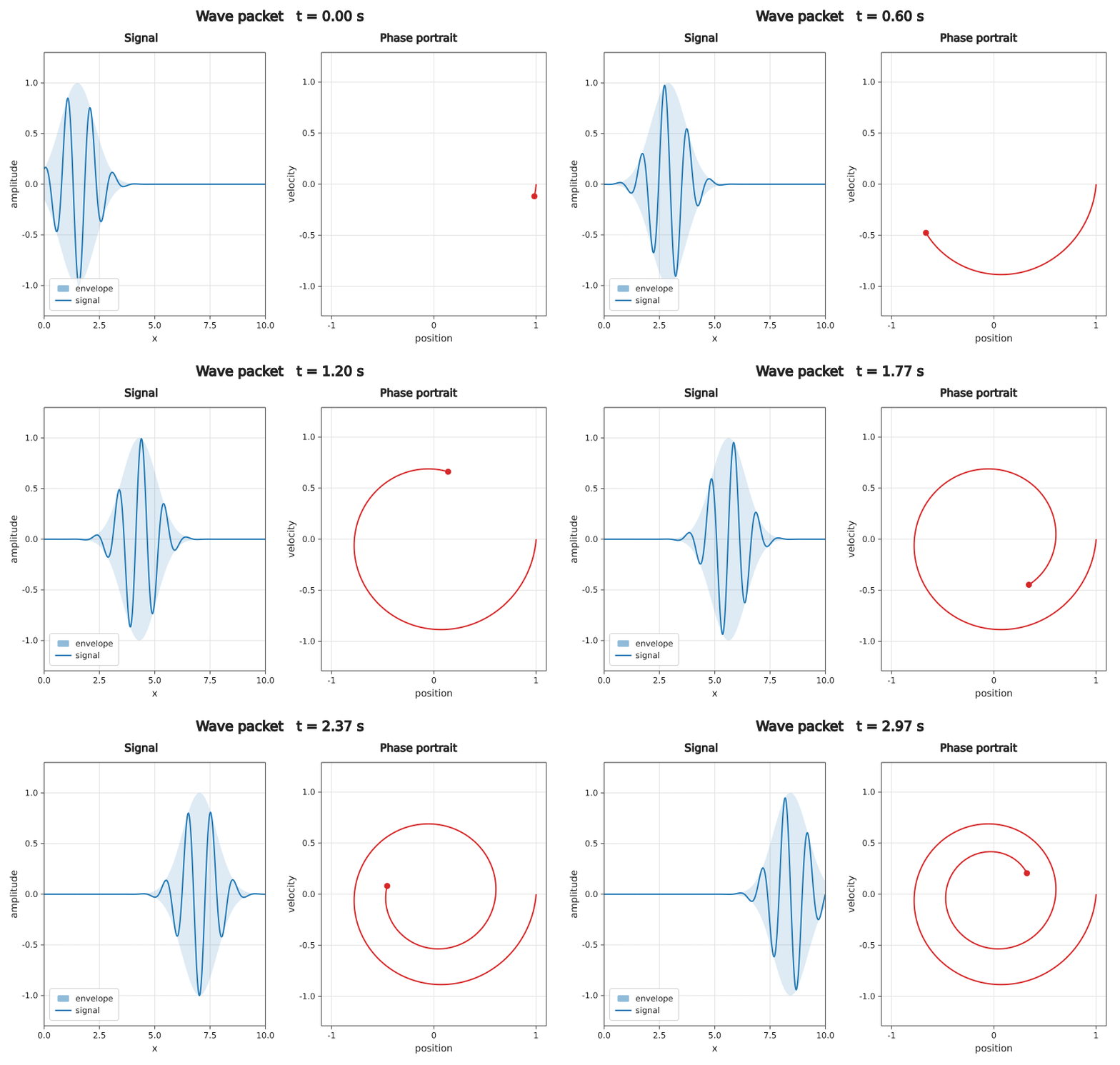
fig.record("wave.gif", 30.0, 120, |fig, i| { /* change the figure */ })?; // .gif .png (APNG) .mp4 .webm
fig.print()?;                      // terminal (colored half blocks or Braille)
fig.render_into(&mut pixels)?;     // RGBA pixels for your own window or texture
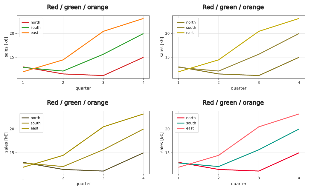
Accessibility
let text = fig.alt_text();          // "Sales. Line chart; quarter from …; Series: north (3 to 5); …"
for w in fig.color_warnings() { println!("{w}"); }   // e.g. two series look alike with deuteranopia
pixels.simulate(Cvd::Deuteranopia); // see the chart as people with color blindness do
SVG, PDF and HTML output carry the title and description for screen
readers.
Backends
fig.backend(Backend::Auto);                // default: CPU, all cores from 1 megapixel on
fig.backend(Backend::Cpu { threads: 1 });  // least CPU time and memory
fig.backend(Backend::Cpu { threads: 0 });  // all cores: lowest latency without a GPU
fig.backend(Backend::Gpu);                 // `gpu` feature: Vulkan / Metal / DX12 / OpenGL
Performance
Measured against matplotlib (Python) and the Rust libraries plotters, ruviz, kuva and charts-rs: the same charts, separate processes, medians (Intel(R) Core(TM) Ultra 7 255HX, NVIDIA GeForce RTX 5070 Ti Laptop GPU, Linux). Full results, method and the code to rerun them: dataviz-examples/benchmarks.
Compared with matplotlib: 8–53× faster for charts saved to PNG, 29× faster for a live 100 000-point chart, and 143× less memory for 10 M points.
Charts to an 800×600 PNG (one thread, time per chart):
| Chart | dataviz | plotters | ruviz | kuva | charts-rs | matplotlib |
|---|---|---|---|---|---|---|
| line, 1 000 points | 1.53 ms | 1.69 ms | 3.58 ms | 5.09 ms | 11.6 ms | 30.2 ms |
| bar, 20 bars | 0.82 ms | 0.84 ms | 3.83 ms | 3.66 ms | 2.15 ms | 43.1 ms |
| scatter, 10 000 points | 2.26 ms | 2.93 ms | 4.29 ms | 8.86 ms | 78.6 ms | 38.7 ms |
| scatter, 100 000 points | 10.2 ms | 17.0 ms | 18.0 ms | 18.0 ms | 808.3 ms | 83.8 ms |
| line, 100 000 points | 2.21 ms | 6.12 ms | 8.08 ms | 29.1 ms | 861.2 ms | 52.2 ms |
| histogram, 1 M values | 2.16 ms | 2.83 ms | 30.3 ms | 16.6 ms | 13.2 ms | 50.8 ms |
Big data (time / memory above the data itself):
| Chart | dataviz | dataviz all cores | plotters | ruviz | kuva | charts-rs | matplotlib |
|---|---|---|---|---|---|---|---|
| line, 10 M points | 126.8 ms / +8 MB | 106.2 ms / +8 MB | 491.9 ms / +315 MB | 330.8 ms / +389 MB | 2.78 s / +787 MB | fails | 597.0 ms / +1162 MB |
| scatter, 10 M points | 236.4 ms / +9 MB | 183.2 ms / +8 MB | 1.64 s / +12 MB | 1.30 s / +377 MB | 1.61 s / +788 MB | fails | 5.16 s / +910 MB |
| histogram, 100 M values | 240.0 ms / +8 MB | 239.9 ms / +7 MB | 247.2 ms / +12 MB | 3.72 s / +1915 MB | 1.67 s / +1551 MB | 1.26 s / +1532 MB | 535.0 ms / +13 MB |
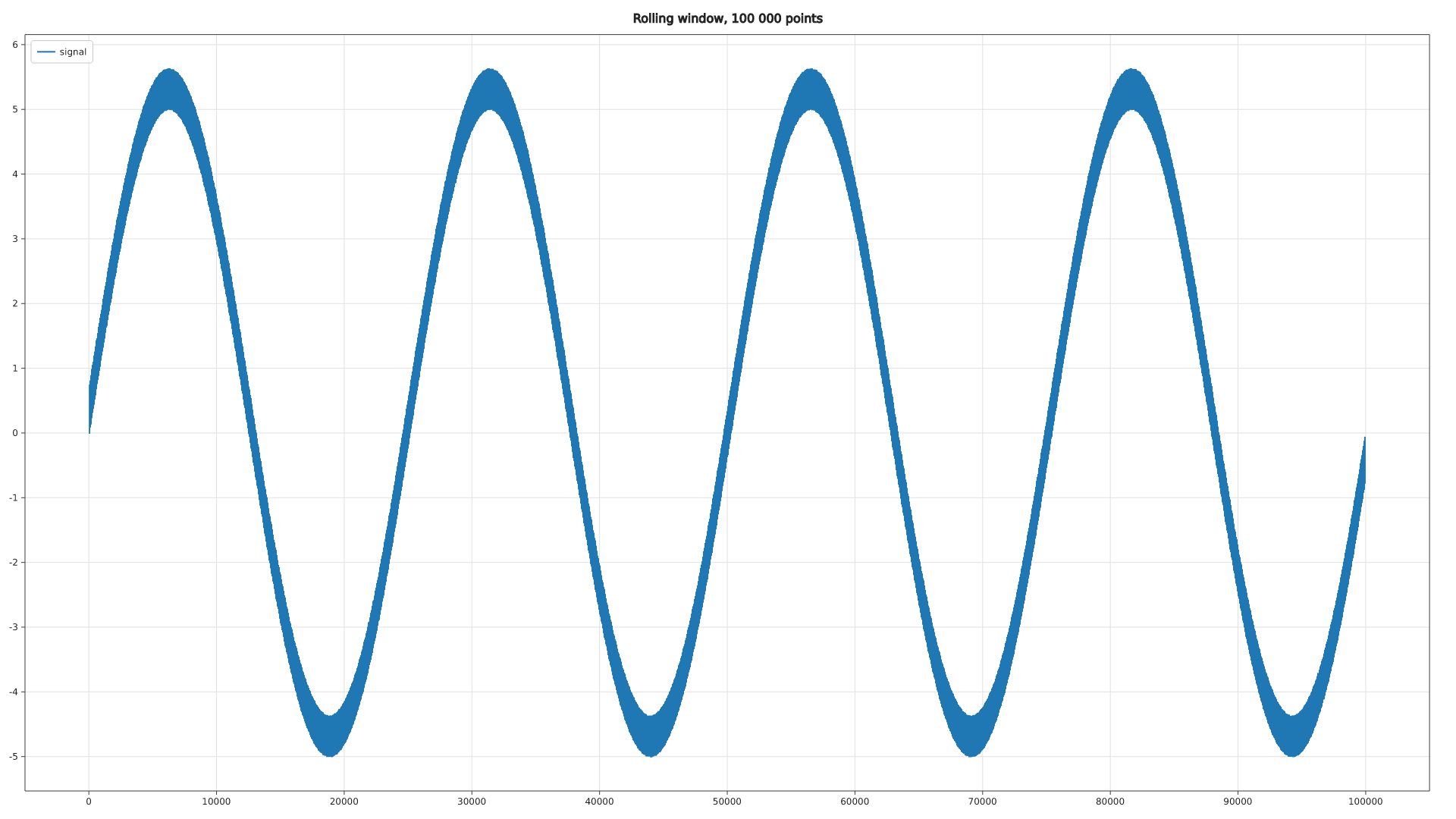
Live chart (rolling window, one new point and a full redraw per frame; latency p50 / CPU per frame / memory of the process):
| Window | dataviz 1 thread | dataviz all cores | dataviz GPU | plotters | ruviz | kuva | matplotlib |
|---|---|---|---|---|---|---|---|
| 1 000 points, 800×600 | 0.78 ms / 0.77 ms / 8 MB | 0.50 ms / 2.60 ms / 9 MB | 0.67 ms / 0.40 ms / 239 MB | 0.65 ms / 0.63 ms / 14 MB | 5.33 ms / 5.33 ms / 11 MB | 5.44 ms / 5.43 ms / 27 MB | 10.1 ms / 10.2 ms / 73 MB |
| 100 000 points, 800×600 | 2.15 ms / 2.13 ms / 12 MB | 1.99 ms / 4.60 ms / 13 MB | 1.73 ms / 1.30 ms / 243 MB | 5.53 ms / 5.53 ms / 16 MB | 33.3 ms / 33.3 ms / 18 MB | 47.5 ms / 47.5 ms / 36 MB | 61.4 ms / 61.5 ms / 112 MB |
| 1 000 points, 1920×1080 | 1.67 ms / 1.70 ms / 16 MB | 0.82 ms / 5.87 ms / 18 MB | 1.52 ms / 1.30 ms / 245 MB | 1.48 ms / 1.50 ms / 18 MB | 17.4 ms / 17.4 ms / 18 MB | 18.1 ms / 18.2 ms / 33 MB | 12.0 ms / 11.9 ms / 79 MB |
| 100 000 points, 1920×1080 | 5.37 ms / 5.40 ms / 19 MB | 3.26 ms / 14.4 ms / 22 MB | 2.82 ms / 2.50 ms / 250 MB | 8.45 ms / 8.47 ms / 21 MB | 121.9 ms / 121.5 ms / 29 MB | 117.8 ms / 117.8 ms / 42 MB | 139.3 ms / 140.1 ms / 177 MB |
Animated GIF (800×600, 120 frames; time, file size):
| Animation | dataviz | plotters | ruviz | matplotlib |
|---|---|---|---|---|
| whole plot moves | 301.0 ms, 1001 KB | 995.0 ms, 3227 KB | 3.87 s, 1741 KB | 5.45 s, 1119 KB |
| line grows on fixed axes | 84.0 ms, 38 KB | 2.98 s, 3257 KB | 4.00 s, 1701 KB | 6.53 s, 420 KB |
3D charts (800×600 PNG; dataviz, plotters and matplotlib on one core, PyVista on the GPU; a rotation frame is the camera turned and the image drawn again):
| Chart | dataviz | dataviz GPU | plotters | matplotlib | PyVista |
|---|---|---|---|---|---|
| surface 60² | 6.03 ms | 5.58 ms | 6.27 ms | 59.3 ms | 100.0 ms |
| surface 200² | 30.5 ms | 50.7 ms | 23.6 ms | 165.2 ms | 113.3 ms |
| scatter 10,000 | 2.99 ms | 1.88 ms | 3.56 ms | 108.2 ms | 95.3 ms |
| scatter 1,000,000 | 148.8 ms | 110.8 ms | 185.8 ms | 6.04 s | 122.6 ms |
| line 100,000 (Lorenz) | 28.3 ms | 13.9 ms | 9.12 ms | 64.0 ms | 91.7 ms |
| molecule 1BNA (486 atoms) | 9.12 ms | 5.87 ms | 2.02 ms | 40.7 ms | 85.6 ms |
| rotation frame: surface 60² | 5.18 ms | 4.90 ms | 5.37 ms | 27.0 ms | 0.66 ms |
| rotation frame: molecule | 7.90 ms | 4.66 ms | 0.95 ms | 12.5 ms | 0.67 ms |
| GIF, 90 frames turning | 915.0 ms, 3649 KB | 1.11 s, 3182 KB | 3.02 s, 4544 KB | 7.97 s, 5713 KB | 4.16 s, 3441 KB |
What makes it fast: the scene is drawn straight into the output buffer by
dataviz's own anti-aliased rasterizer; dense lines become one pixel-column
envelope and dense scatter plots an occupancy grid, so time and memory stay
flat as the data grows; data passed to a series is not copied; glyphs and
markers are cached as bitmaps; histograms use SIMD binning. Animations store
only the changed part of each frame. On the web the same renderer compiled to
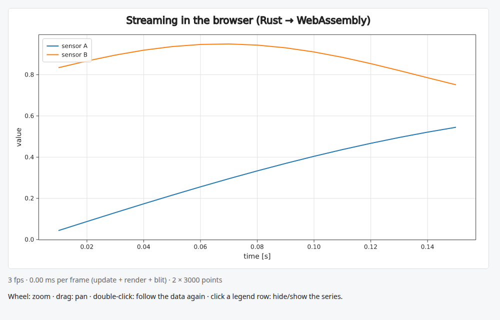
WebAssembly draws a 960×520 live chart with 2 × 3 000 points in about 1.7 ms.
In 3D dataviz is 36–41× faster than matplotlib for scatter plots, 5–10×
for surfaces and 1.6–5× for lines, molecules and rotation frames; it draws
a turning GIF 3.3× faster than plotters and 4.5× faster than PyVista and
is first (on the CPU or the GPU) for the 60² surface and for scatter plots
up to a million points, with lighting, depth order and anti-aliasing.
plotters is faster for the large surface, the long 3D line and the
molecule: it draws 1-pixel lines and flat circles without depth sorting or
lighting. PyVista (VTK) keeps the scene on the GPU and turns it in 0.7 ms
per frame against dataviz's 5–8 ms (still 125–200 frames per second), but
needs 85–115 ms to save an image and about 300 MB of memory.
Where it is not first: for a tiny live chart (1 000 points) on a single
thread plotters is 0.1–0.2 ms faster per frame; dataviz on all cores is
the fastest there. The GPU backend needs the least CPU time but ~240 MB of
driver memory and ~0.3 s to start, so the default stays on the CPU.
Gallery
Every image links to its example in
dataviz-examples (code,cargo run, output).
Live, interactive and animated
For data scientists, biologists, engineers and traders
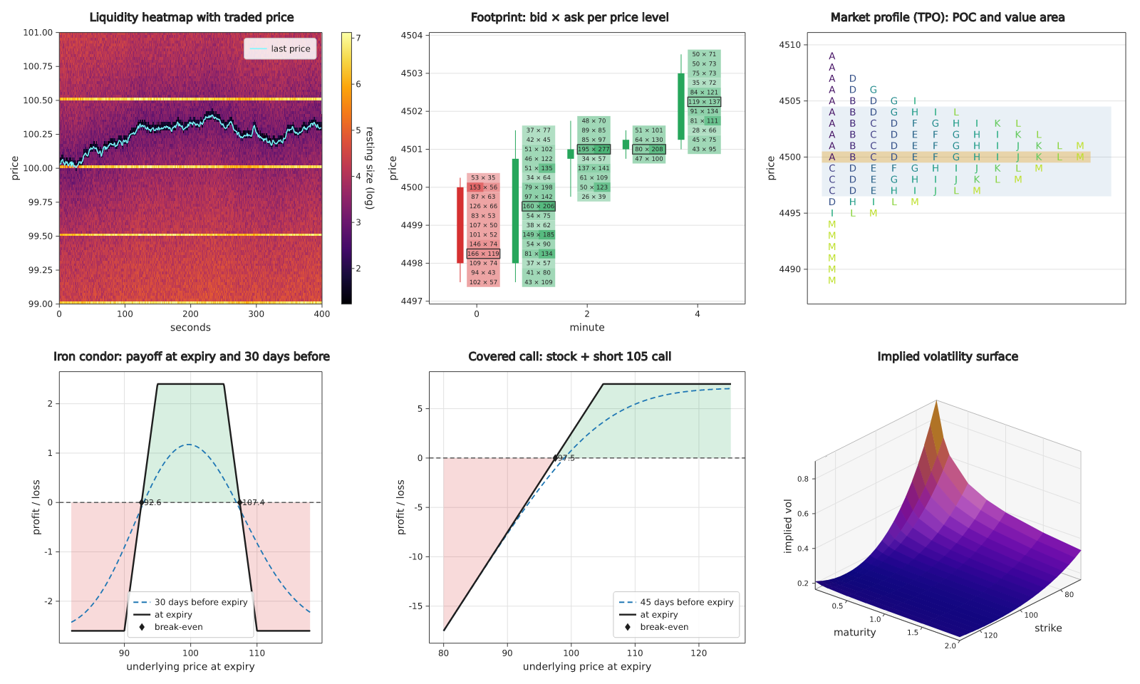
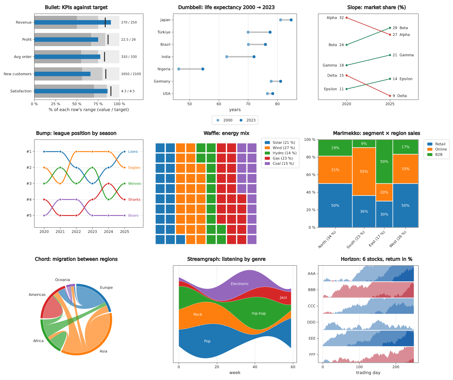
Lines, points and bars
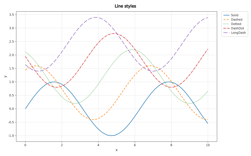 Line styles | 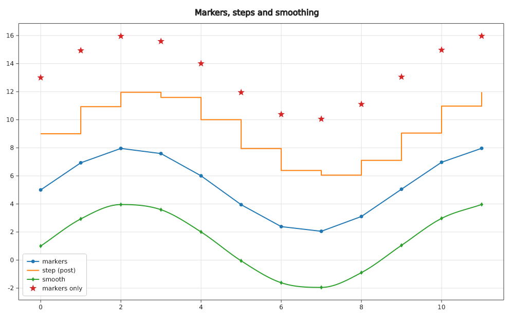 Markers, steps and smoothing | 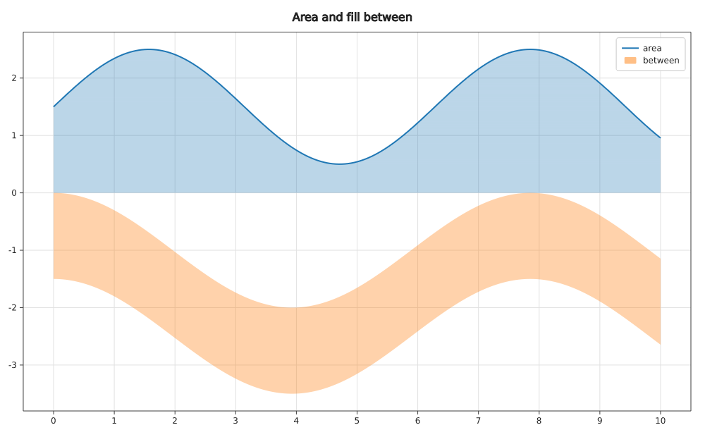 Area and fill between |
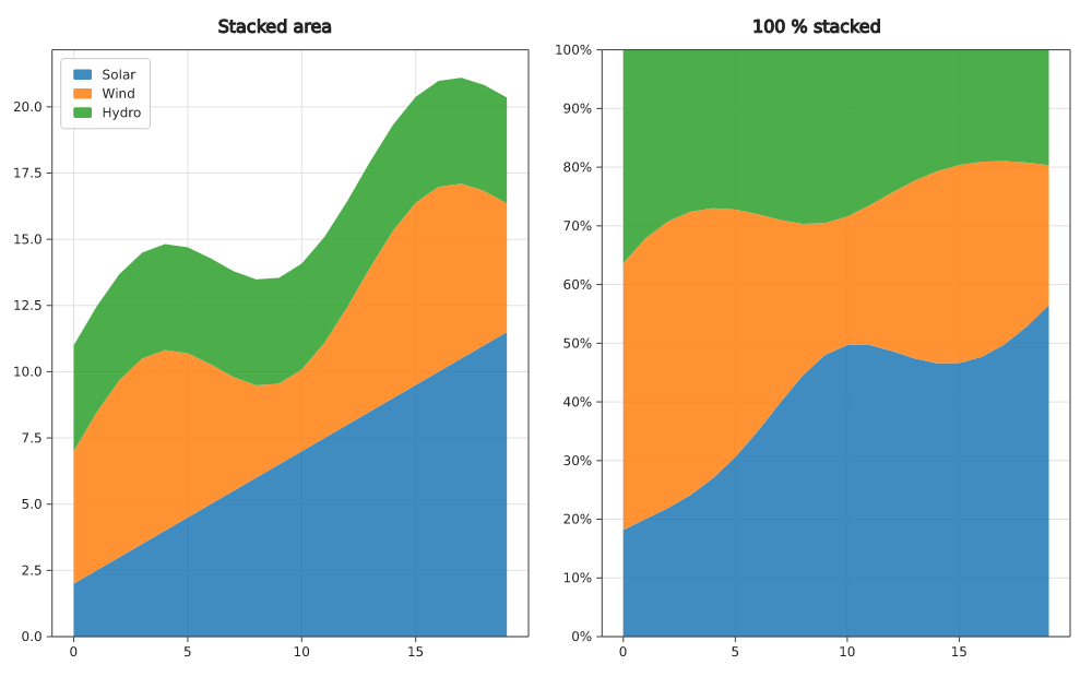 Stacked areas | 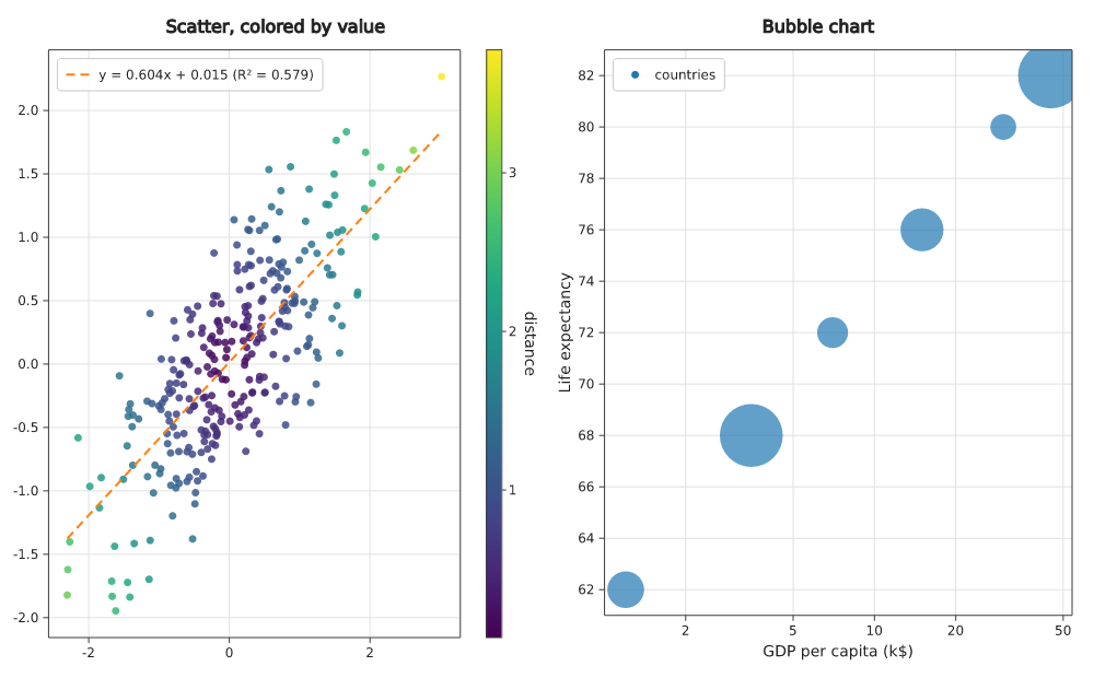 Scatter and bubble charts | 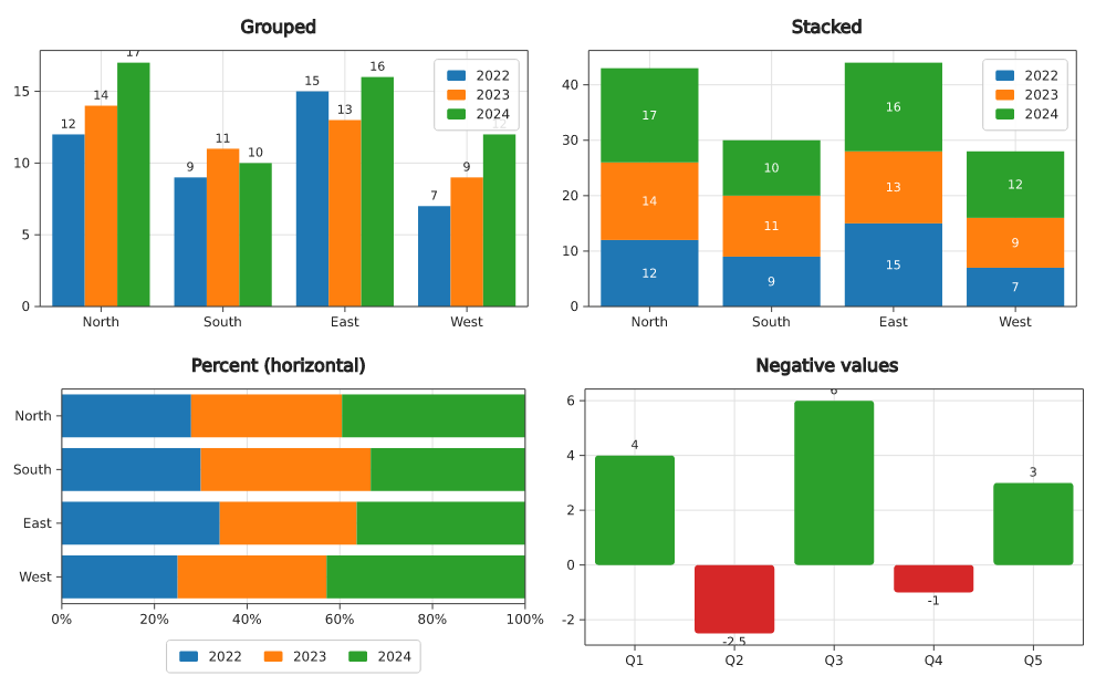 Bar charts |
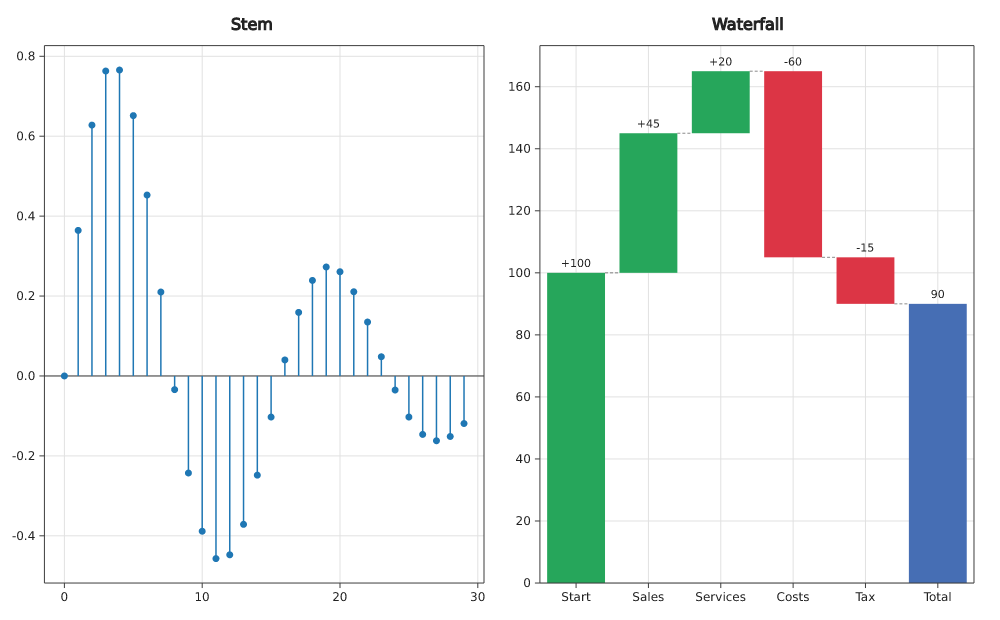 Stem and waterfall charts | 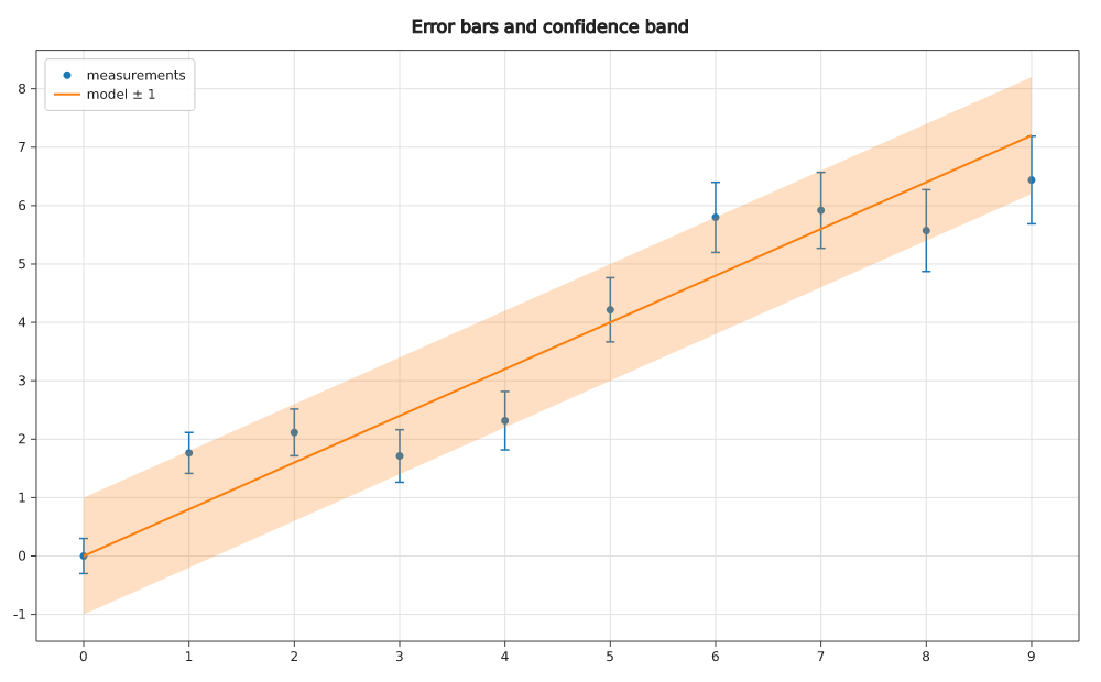 Error bars and confidence bands | 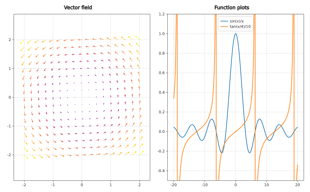 Vector field and function plots |
Statistics
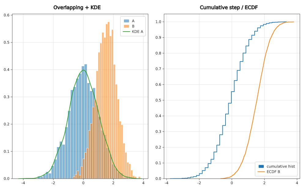 Histograms, KDE and ECDF | 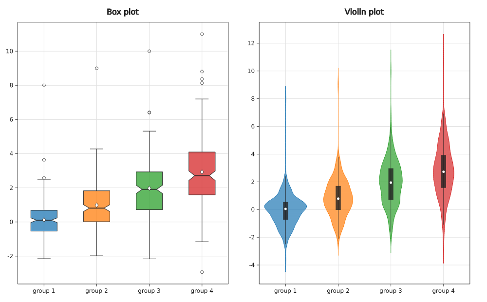 Box and violin plots | 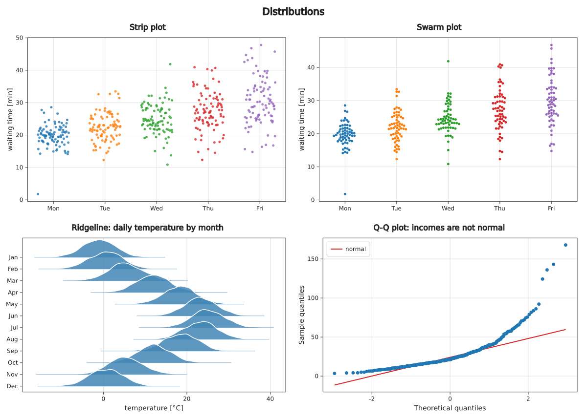 Strip, swarm, ridgeline, Q-Q |
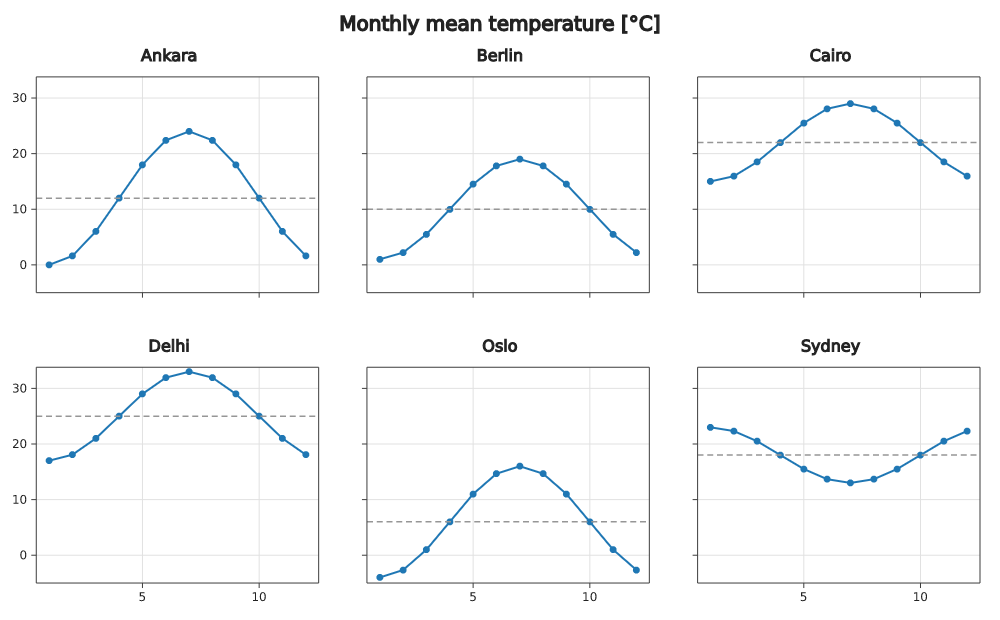 Facets (small multiples) | 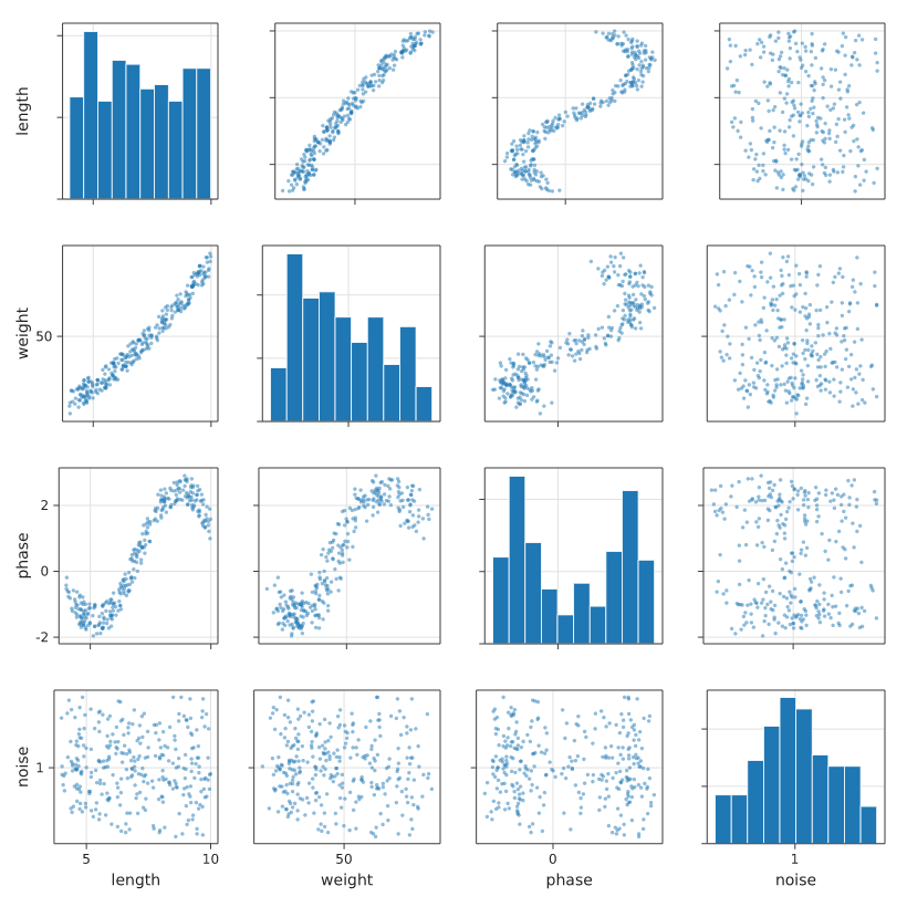 Pair plot (scatter matrix) | 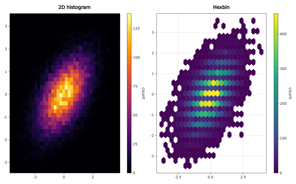 2D histogram and hexbin |
Finance and time
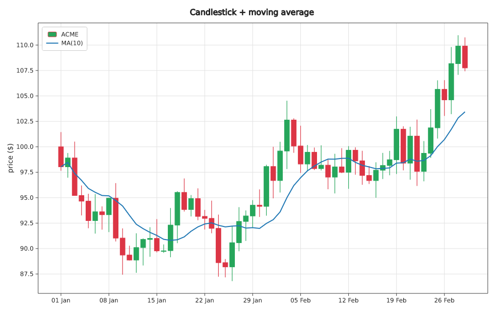 Candlestick chart | Bollinger, RSI, MACD | 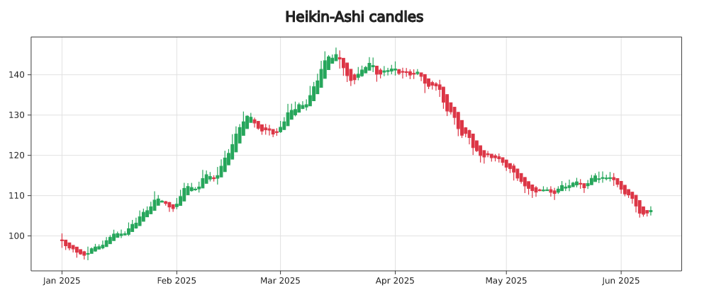 Heikin-Ashi candles |
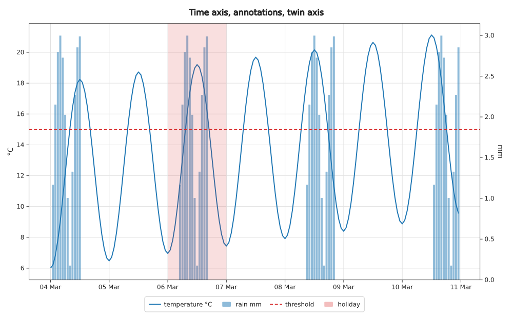 Time series | 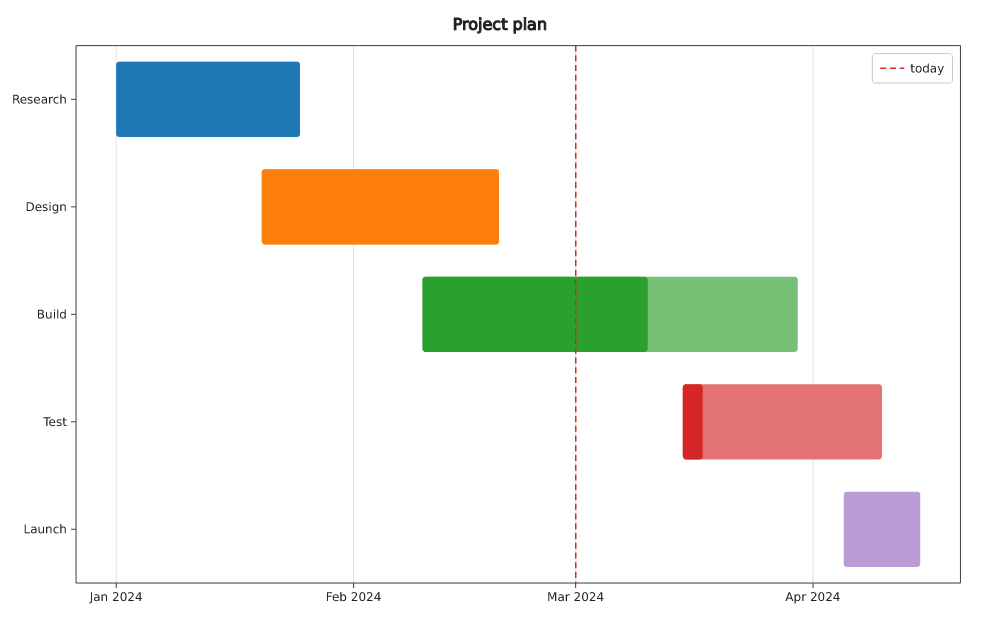 Gantt chart | 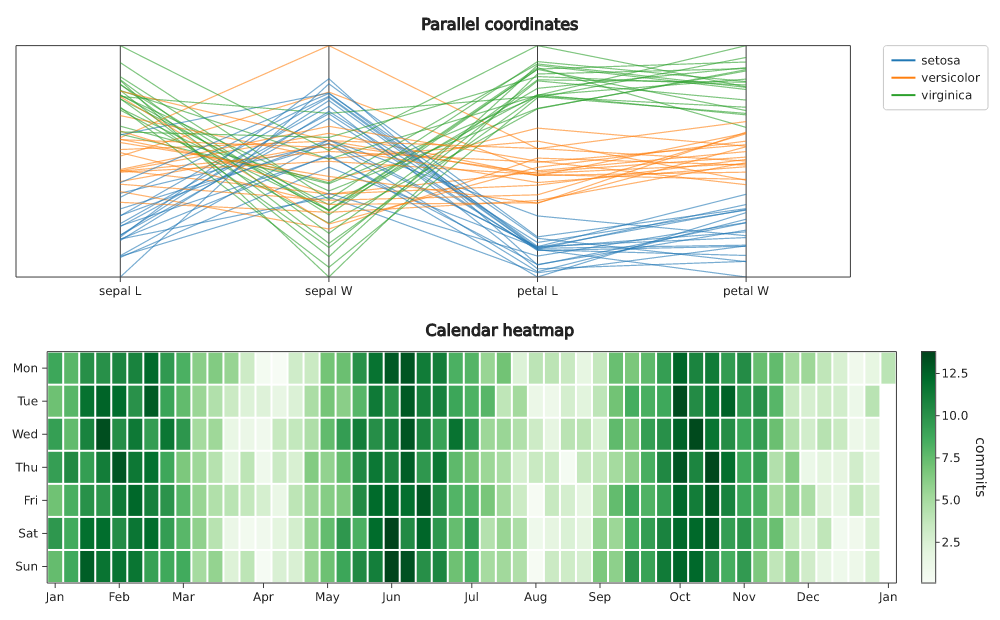 Parallel coordinates and calendar |
Grids, fields and 3D
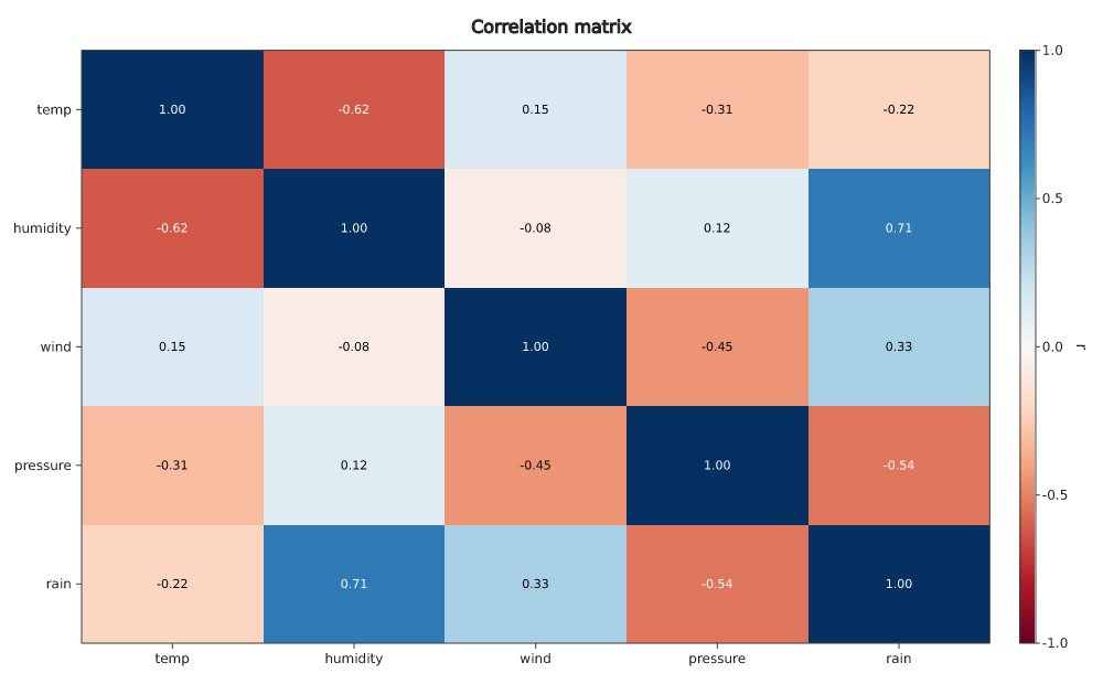 Heatmap (correlation matrix) | 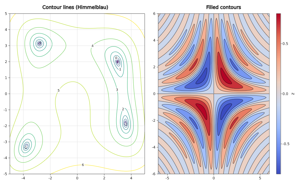 Contour plots | 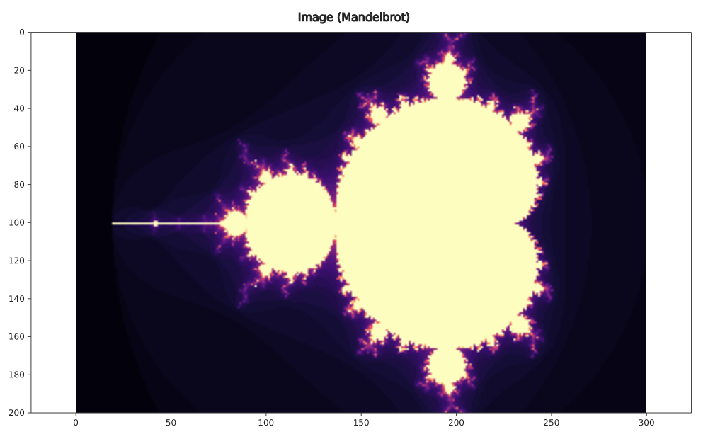 Images |
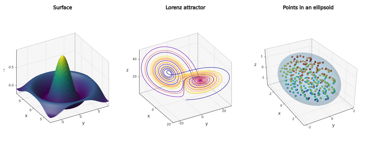 3D surface, Lorenz attractor, mesh |
Maps
Choropleth and flight routes | 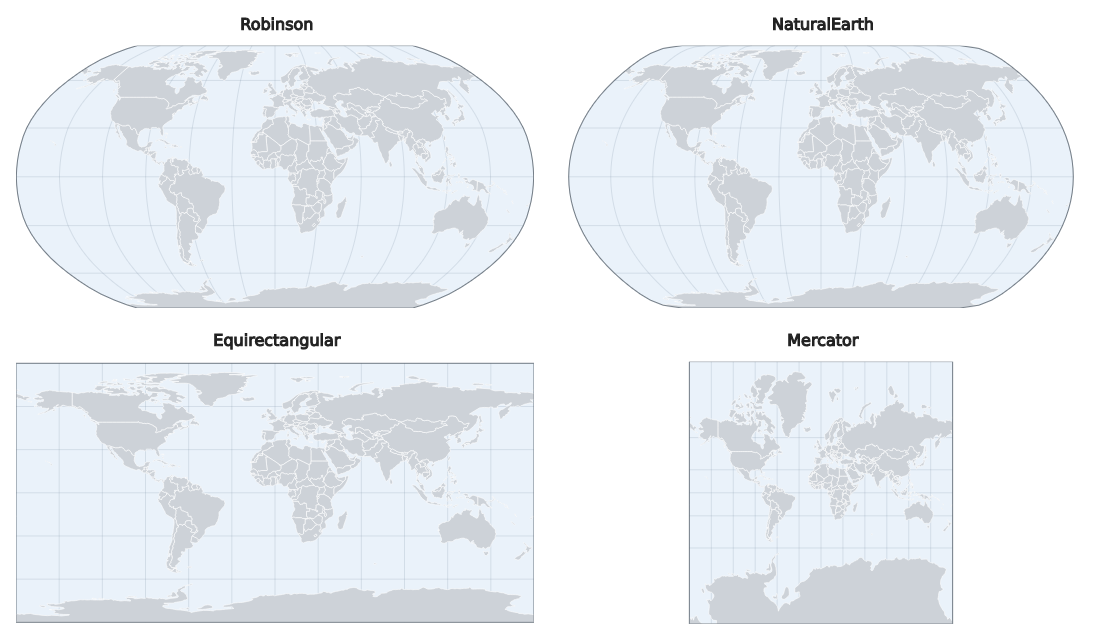 Map projections |
Parts, flows and polar
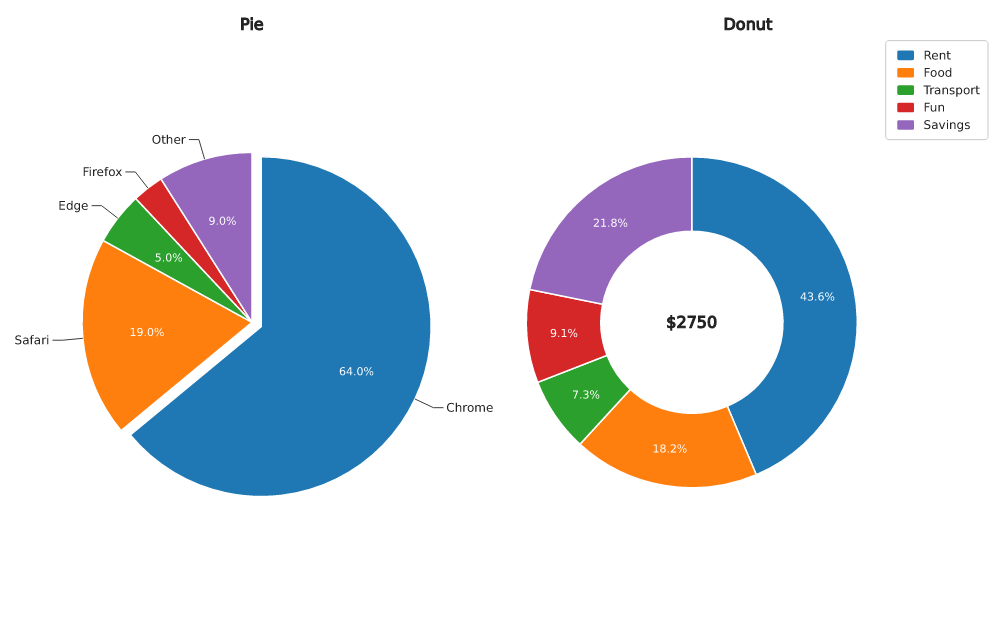 Pie and donut charts | 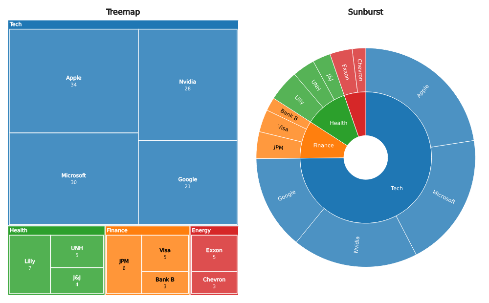 Treemap and sunburst | 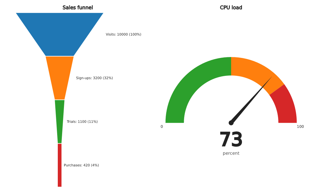 Funnel and gauge |
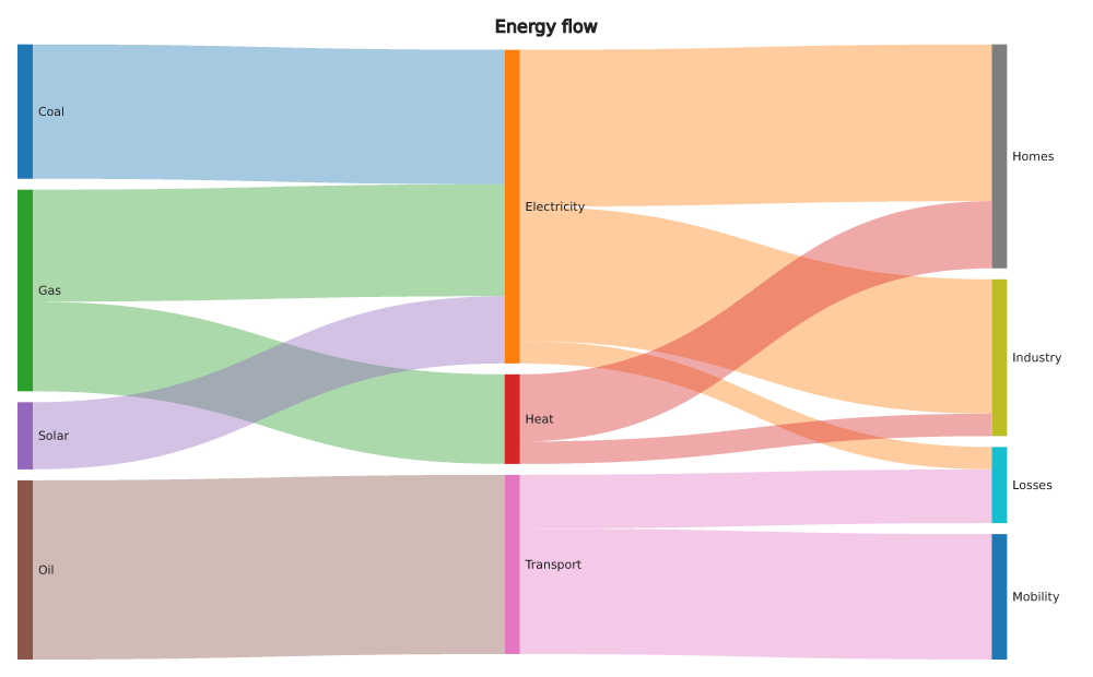 Sankey diagram | 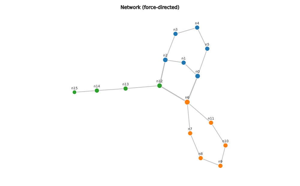 Network graph | 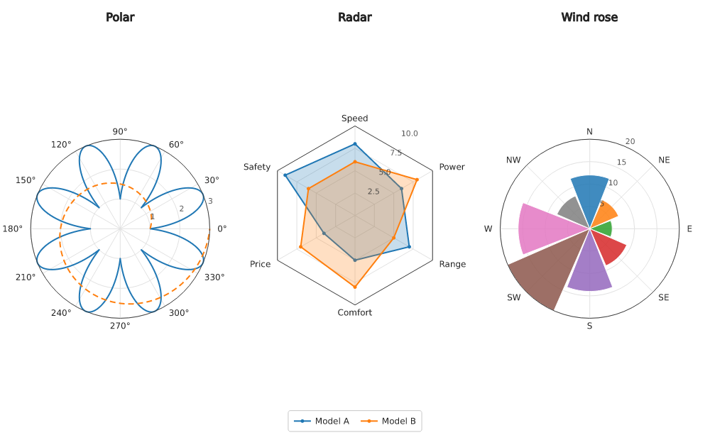 Polar and radar charts |
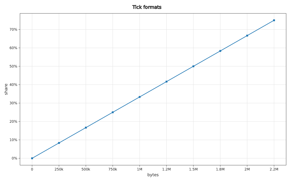
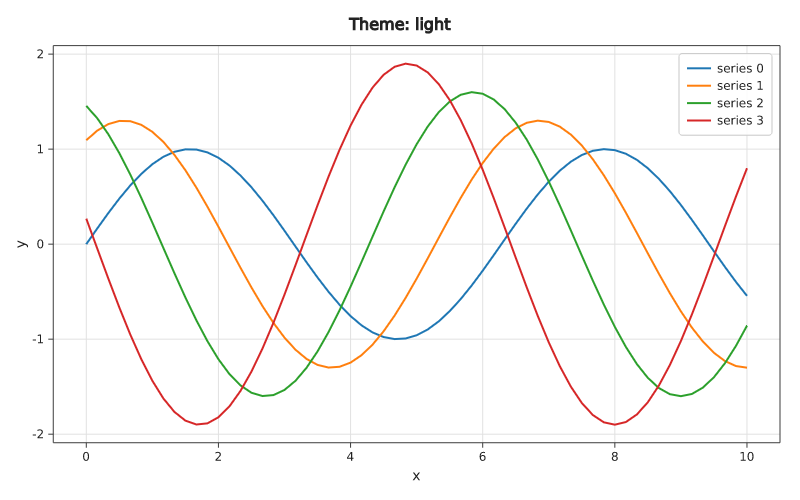
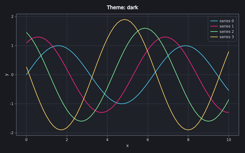
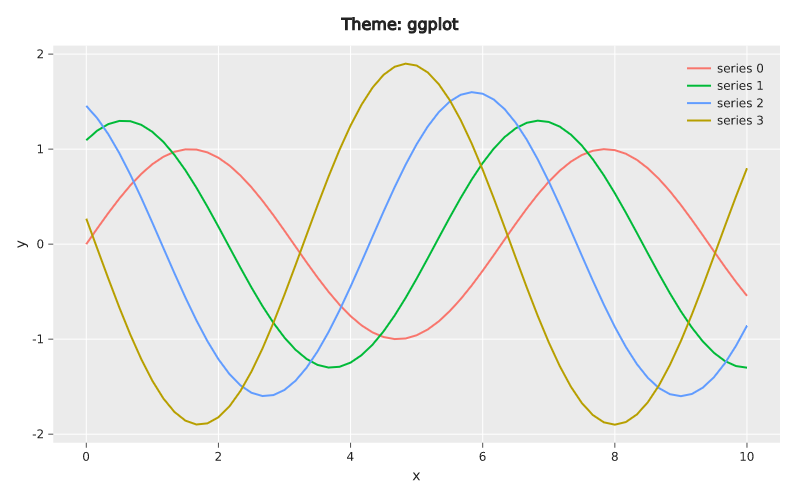
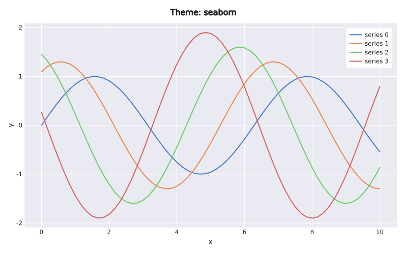
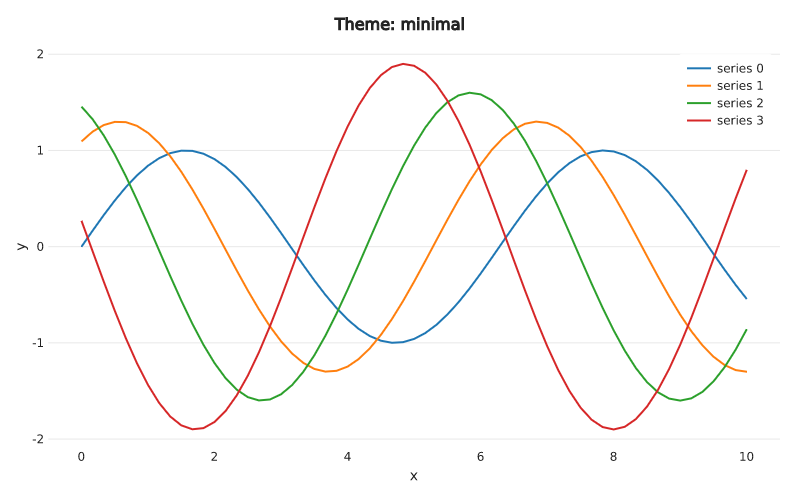
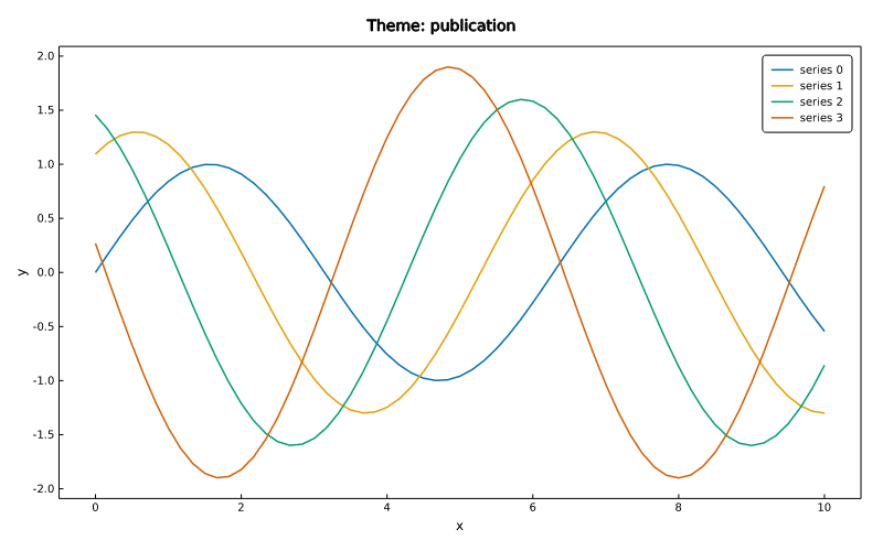
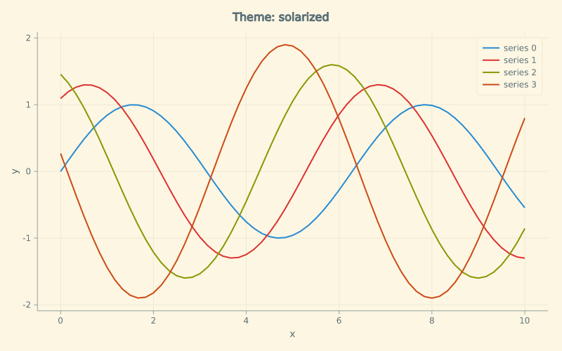
Axes, layout, text and style
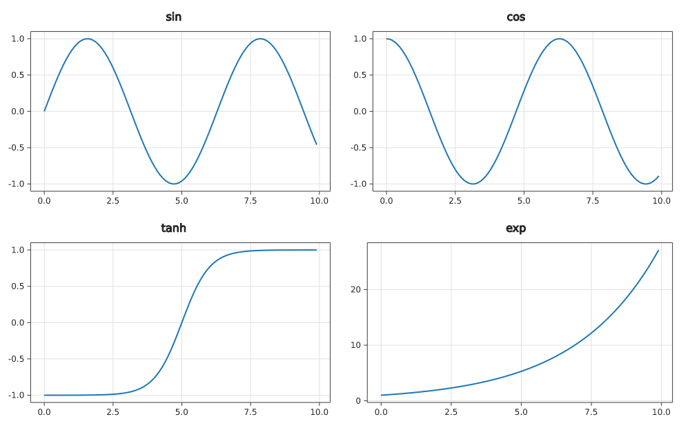
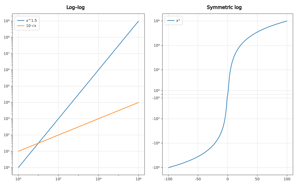
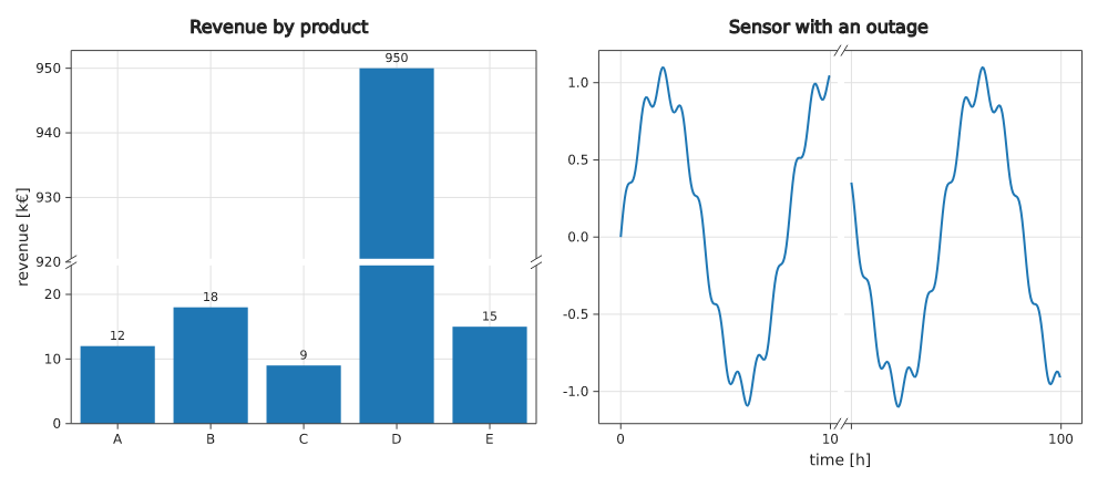
Python
The same renderer for Python (python/): NumPy, pandas and
Polars data, Jupyter display, 5–22× faster than matplotlib.
import numpy as np, dataviz as dv
x = np.linspace(0, 10, 100_000)
fig = dv.Figure(900, 500, title="Signal")
fig.axes().line(x, np.sin(x), label="sin").set(x_label="t [s]")
fig.save("signal.png")
Use it from Claude
The Claude Code plugin gives Claude all of these charts:
it draws from your data, CSV/JSON files and PDB structures, looks at the
image and refines it.
/plugin marketplace add dataviz-rs/dataviz
/plugin install dataviz@dataviz
Then ask: "plot bench.csv and compare the branches", "show 1UBQ as a
cartoon with its Ramachandran plot", or use /dataviz:plot and/dataviz:molecule. Other MCP clients use the server directly:cargo install dataviz-mcp (dataviz-mcp).
Installation
[dependencies]
dataviz = "0.15"
# dataviz = { version = "0.15", features = ["pdf", "gpu"] }
# dataviz = { version = "0.15", default-features = false }   # headless / wasm32
| Feature | Default | What it adds |
|---|---|---|
window |
yes | interactive windows (minifb) |
pdf |
no | PDF output |
gpu |
no | GPU rasterization (wgpu) |
Requires Rust 1.89 or newer. On Linux the window feature needs the usual
windowing libraries (libxkbcommon-dev, libwayland-dev).
Changelog
See CHANGELOG.md.
License
MIT; see LICENSE. The embedded DejaVu Sans font has its own license
(assets/DejaVuSans-LICENSE.txt); the world map is Natural Earth (public
domain).
Contributing
Bug reports, ideas and pull requests are welcome at
https://github.com/dataviz-rs/dataviz.
Yorumlar (0)
Yorum birakmak icin giris yap.
Yorum birakSonuc bulunamadi