SpiceMCP
Health Uyari
- No license — Repository has no license file
- Description — Repository has a description
- Active repo — Last push 0 days ago
- Low visibility — Only 7 GitHub stars
Code Gecti
- Code scan — Scanned 12 files during light audit, no dangerous patterns found
Permissions Gecti
- Permissions — No dangerous permissions requested
Bu listing icin henuz AI raporu yok.
LTspice MCP server where the server owns the optimization state, not the LLM.
SpiceMCP
LTspice MCP server where the server owns the optimization state, not the LLM.
The model contributes topology and strategy. Candidate identity, simulation history,
dedup, best so far, sensitivities and rollback all live in SQLite and are re derived
on every call, so a long optimization can't drift into remembering a circuit that
never existed.
Prototype Status & Live Example
SpiceMCP is currently an experimental prototype.
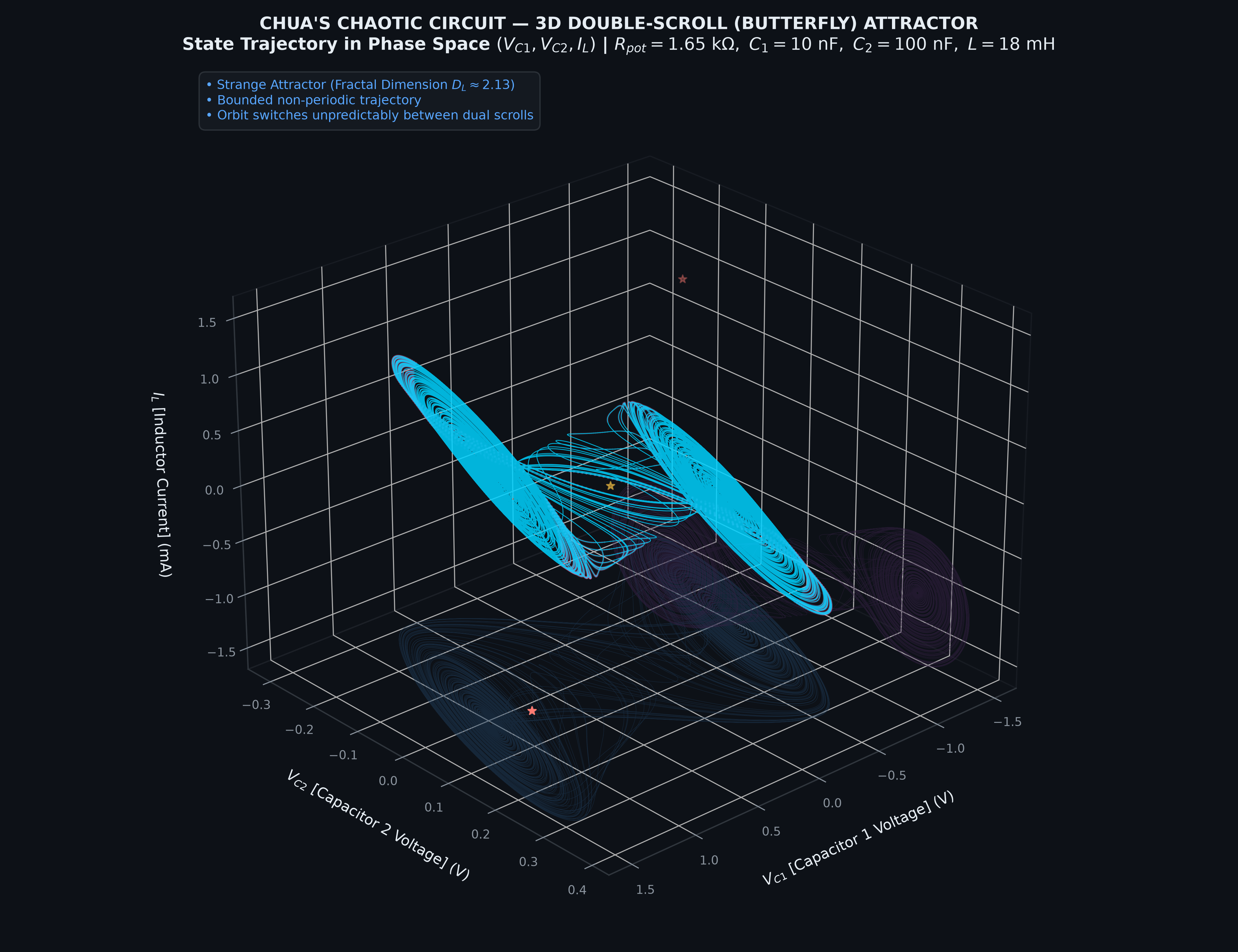
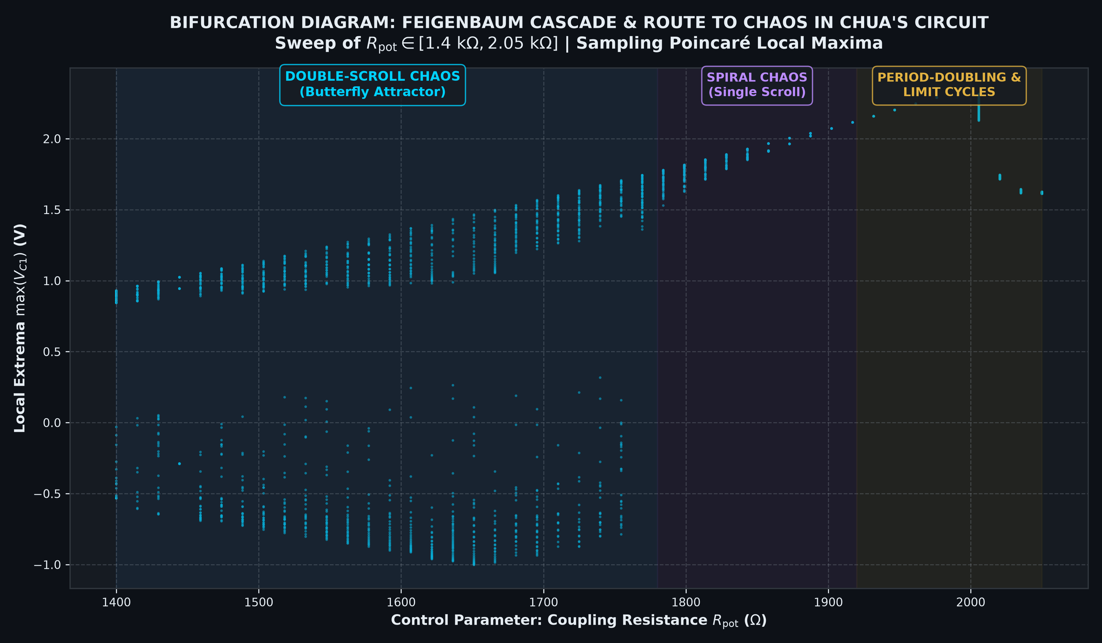
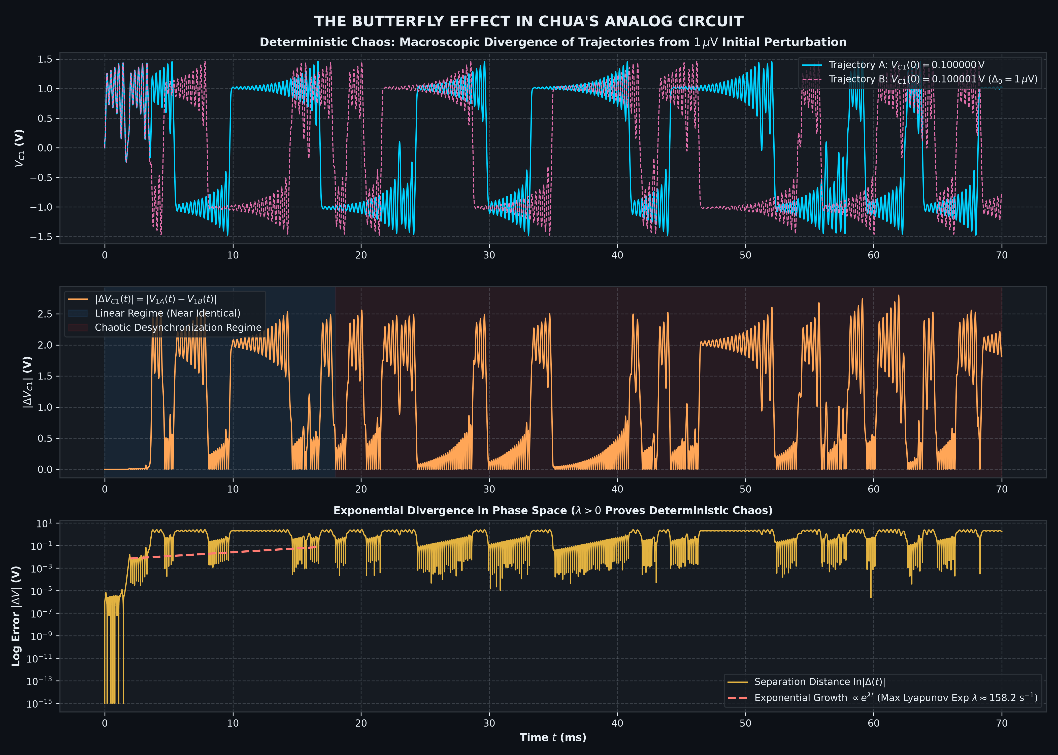
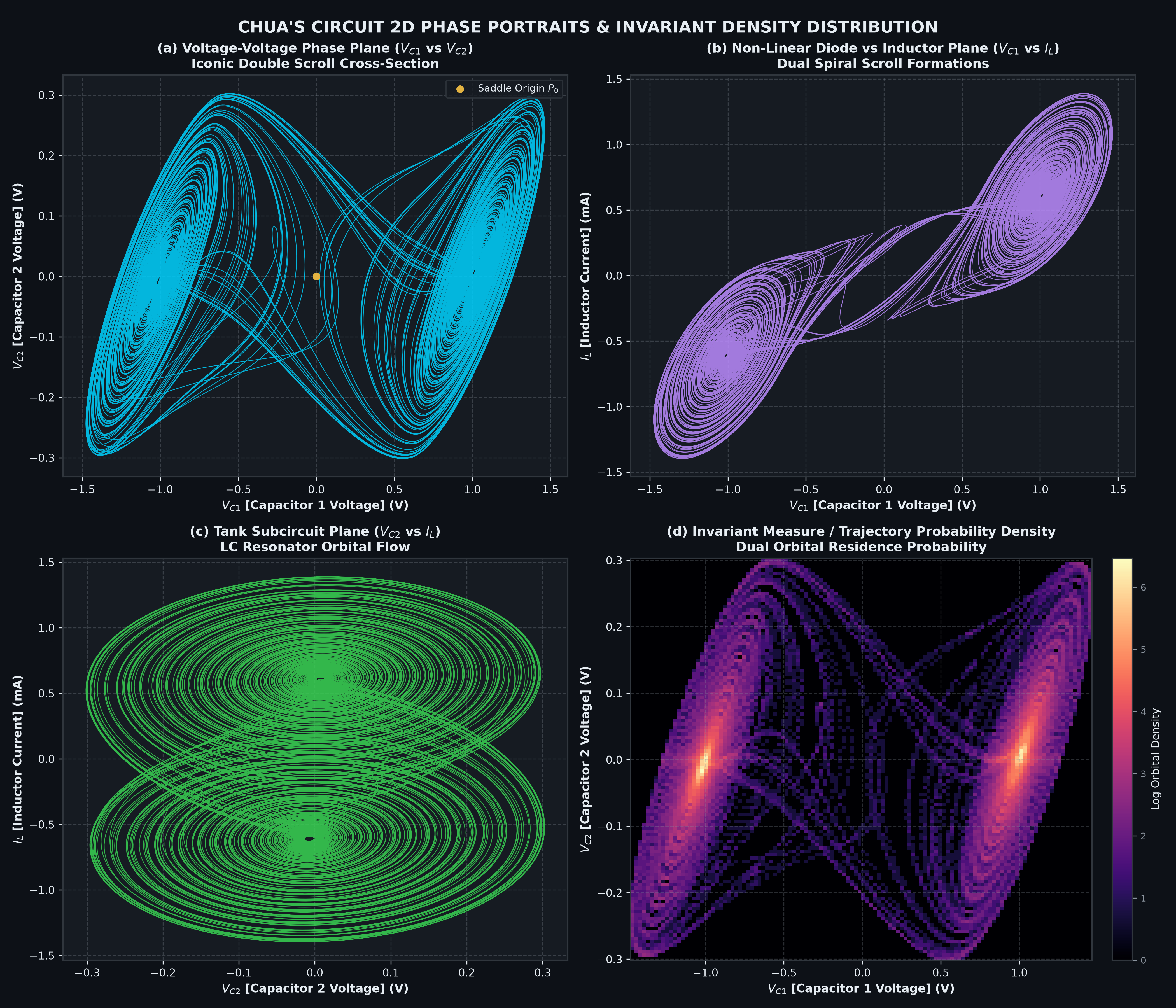
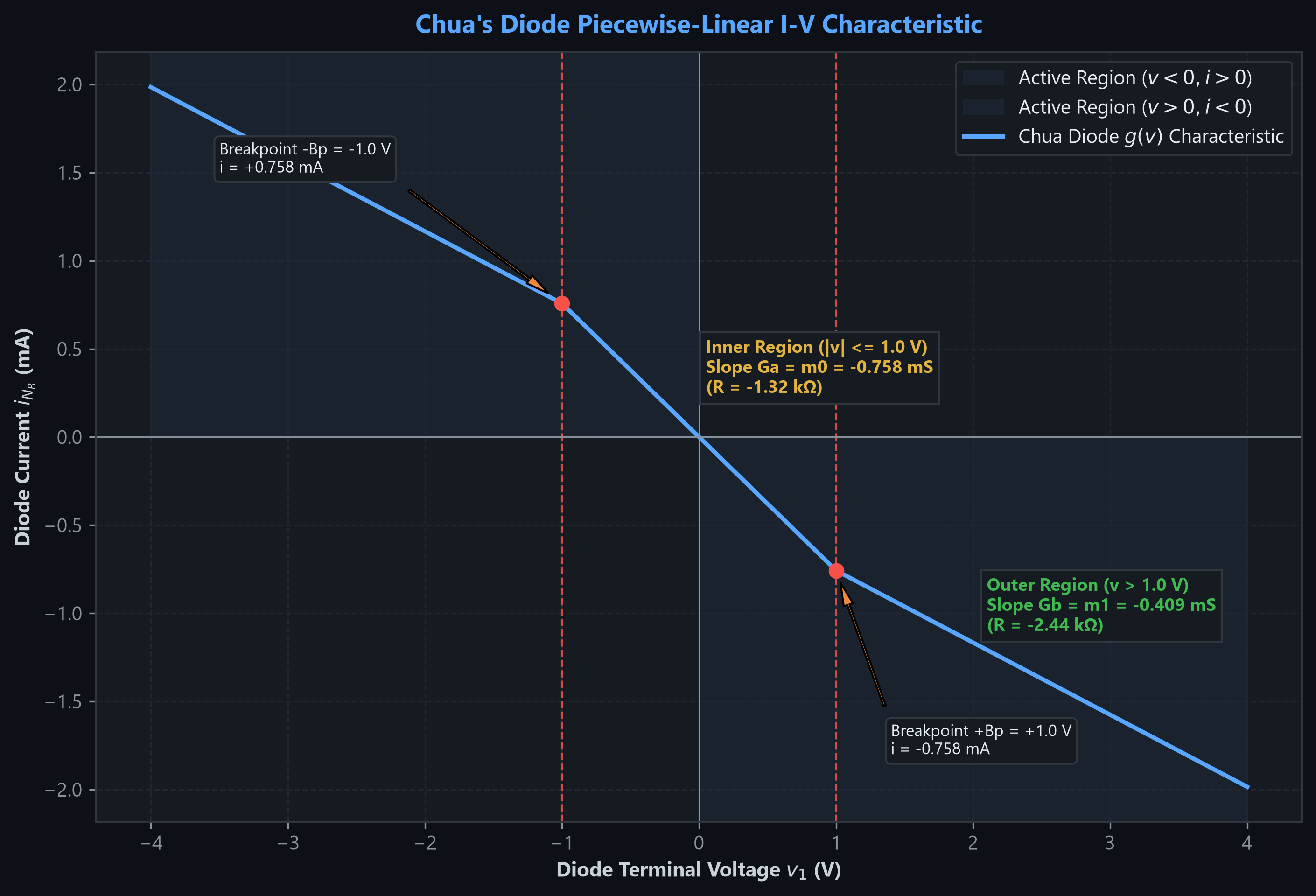
Below is a demonstration of what SpiceMCP generated and analyzed autonomously for Chua's Chaotic Circuit showcasing automated
.ascschematic generation, batch LTspice simulations, binary.rawwaveform parsing, parameter sweeps, and visualization:
Schematic Rendering ( render_schematic)3D Double-Scroll Attractor Vector schematic generated from .ascinclassicstyle3D phase-space trajectory $(v_{C1}, v_{C2}, i_L)$ parsed from binary .raw
Bifurcation Route to Chaos ( simulatesweep)Sensitivity to Initial Conditions (Butterfly Effect) Multi-point parameter sweep capturing period-doubling cascades Lyapunov divergence tracking $1,\mu\text{V}$ initial condition perturbations
2D Phase Plane Portraits & Orbital Density Nonlinear Diode (NDR) I-V Curve Orthogonal projections ($V_{C1}-V_{C2}, V_{C1}-I_L$) with orbital density Piecewise-linear Negative Differential Resistance ($G_a, G_b$) DC sweep
Architecture
flowchart TB
    subgraph Client ["LLM / MCP Client"]
        Agent["AI Agent / LLM<br/><i>(Topology & Optimization Strategy)</i>"]
    end

    subgraph Server ["SpiceMCP Server (FastMCP API)"]
        direction TB
        subgraph ToolEndpoints ["Tool Endpoints (11 Tools)"]
            T_Life["<b>Lifecycle Tools</b><br/>start_optimization<br/>stop_optimization"]
            T_Eval["<b>Evaluation & Search</b><br/>run_optimization<br/>evaluate_candidate"]
            T_Sim["<b>Simulation & Sweeps</b><br/>simulate"]
            T_Diag["<b>Feasibility & System</b><br/>check_feasibility<br/>check_setup"]
            T_Vis["<b>Schematics</b><br/>render_schematic"]
            T_Query["<b>State Queries & Reports</b><br/>query_run (status / best / pareto /<br/>history / sensitivity / compare / ...)<br/>generate_design_report<br/>rollback_to_candidate"]
        end
    end

    subgraph Core ["Optimization & Circuit Core"]
        Engine["<b>Optimization Engine</b> (engine.py)<br/>• Coordinate descent & step halving<br/>• Pure-function scoring & Pareto frontier<br/>• Empirical sensitivity analysis (FD / OLS)"]
        IR["<b>Circuit IR & Hashing</b> (ir.py)<br/>• Template placeholder substitution: {param}<br/>• Fingerprinting (topology, design, config)<br/>• Deterministic deduplication"]
        ASC["<b>Schematic Writer</b> (asc.py)<br/>• Pin-name routing with symbol (.asy) parsing<br/>• Orthogonal L-routing (HV/VH/auto)<br/>• Round trip netlist validation via asc.check()"]
        Render["<b>Schematic Renderer</b> (render.py)<br/>• Real .asy geometry & transformation matrices<br/>• SVG (zero dependency) and PNG (matplotlib)<br/>• 3 styles: tech_minimal, classic, sketch<br/>• Label collision avoidance"]
        Robust["<b>Robustness & Waves</b> (robustness.py, raw.py)<br/>• DC operating point & bias audit<br/>• PVT corners & Monte Carlo yield / Cpk<br/>• Binary .raw parser & waveform metrics"]
        Feas["<b>Preflight Feasibility</b> (feasibility.py)<br/>• 3 tiers: static, template, physics<br/>• 3 modes: practical, theoretical, concept<br/>• Closed form limits (SR, GBW, noise, filter order)"]
        Rep["<b>Design Report & Plots</b> (report.py, plots.py)<br/>• Six-section Markdown, rendered from state<br/>• BOM, baseline vs final, Bode/tran/THD figures<br/>• Unified 5-color visualization ramp & chrome"]
    end

    subgraph Simulation ["Simulation Layer (sim.py)"]
        Router{"Backend Router"}
        LTSpice["<b>LTspice Executable</b><br/>Batch process (<code>-b -ascii</code>)"]
        Analytic["<b>Analytic Backend</b><br/>Fast closed form surfaces (test/dry-run)"]
        SweepEngine["<b>Sweep Engine</b><br/>Single launch <code>.step</code> multipoint execution<br/>Value recovery from .log / .raw"]
        MeasParser["<b>Log & Meas Parser</b><br/>• .meas regex metric extraction<br/>• Complex AC magnitude/phase parsing<br/>• Failure taxonomy classifier"]
    end

    subgraph State ["Authoritative State (.ltspice-mcp/)"]
        subgraph DB ["SQLite Database (state.db - WAL Mode)"]
            T_Runs[("<b>runs</b><br/>Templates, parameter bounds, objectives")]
            T_Designs[("<b>designs</b><br/>Byte exact netlists, lineages, SHA hashes")]
            T_Exps[("<b>experiments</b><br/>Metrics, scores, feasibility, failures")]
            T_Sens[("<b>sensitivities</b><br/>Slopes, R2, confidence")]
        end
        subgraph FS ["Filesystem Artifacts"]
            CandDir["<code>candidates/</code> (cand_XXXX.cir)"]
            SimDir["<code>simulations/</code> (adhoc, sweep, logs, raw)"]
            RepDir["<code>reports/</code> & <code>plots/</code>"]
        end
    end

    %% Communication Flow
    Agent -->|"1. Tool calls (goals, param space, evaluations)"| ToolEndpoints
    ToolEndpoints -->|"6. Compact summaries, sensitivities, best candidates"| Agent

    T_Life & T_Eval & T_Query --> Engine
    T_Sim --> Router
    T_Diag --> Feas
    T_Diag --> Router
    T_Vis --> Render
    Engine -->|"Refuse impossible specs before any state is written"| Feas
    Engine --> IR
    Engine --> Robust

    Engine -->|"Execute candidate sim"| Router
    Router -->|"Subprocess"| LTSpice
    Router -->|"In-memory"| Analytic
    Router --> SweepEngine
    LTSpice -->|"Parse .log / .raw"| MeasParser
    SweepEngine --> MeasParser
    Analytic --> MeasParser
    MeasParser -->|"Extracted metrics & failure status"| Engine

    IR -->|"Query existing fingerprints"| T_Designs
    Engine -->|"ACID Transaction (append only history)"| DB
    Engine -->|"Store byte exact netlists & traces"| FS
    T_Query -->|"Rederive dynamically (best, pareto, sensitivities)"| DB
    T_Query --> Rep
    Rep -->|"Read stored state, never hand entered numbers"| DB
    Rep -->|"Resimulate the winner for waveforms & corners"| Robust
    Rep -->|"Write DESIGN_REPORT.md + figures"| RepDir
    ASC -.->|"Round trip verification"| LTSpice
    Render -.->|"Parse .asy symbol definitions"| FS

    %% Styling based on SpiceMCP visual style palette
    classDef client fill:#f9f9f9,stroke:#333,stroke-width:2px,color:#333
    classDef endpoint fill:#1E56A0,stroke:#12396e,stroke-width:2px,color:#fff
    classDef core fill:#38A3A5,stroke:#23696a,stroke-width:2px,color:#fff
    classDef sim fill:#E07A5F,stroke:#9c5340,stroke-width:2px,color:#fff
    classDef db fill:#D9534F,stroke:#933734,stroke-width:2px,color:#fff
    classDef fs fill:#F2CC8F,stroke:#a68a5d,stroke-width:2px,color:#333

    class Agent client
    class T_Life,T_Eval,T_Sim,T_Diag,T_Vis,T_Query endpoint
    class Engine,IR,ASC,Render,Robust,Feas,Rep core
    class Router,LTSpice,Analytic,SweepEngine,MeasParser sim
    class T_Runs,T_Designs,T_Exps,T_Sens db
    class CandDir,SimDir,RepDir fs
Install
pip install -e ".[dev]"
pytest -q
LTspice is auto-detected (AppData\Local\Programs\ADI\LTspice\LTspice.exe,Program Files\LTC\LTspiceXVII\XVIIx64.exe, …). Override with LTSPICE_EXE.
Register with your MCP client:
{
  "mcpServers": {
    "spicemcp": {
      "command": "python",
      "args": ["-m", "spicemcp.server"],
      "env": { "SPICEMCP_PROJECT": "C:/path/to/your/circuit/project" }
    }
  }
}
State lands in $SPICEMCP_PROJECT/.ltspice-mcp/:
state.db      authoritative state (SQLite WAL)
candidates/   cand_XXXX.cir, byte exact netlists for rollback
simulations/  LTspice working dirs, logs, and raw waveforms
reports/      Markdown design reports and iteration traces
plots/        Rendered Bode, transient, and THD figures
Metrics come from .meas
Every metric you optimize on is a .meas directive in the netlist, and the server reads
the values back from LTspice's .log. The metric definitions then live with the circuit,
versioned alongside it. Waveforms are a separate concern: spicemcp.raw parses the binary.raw for the report's plots and for a sweep with no .meas, but nothing in the search
loop scores a candidate off a wave.
.ac dec 100 1 10Meg
.meas AC gain_db MAX mag(V(out))          ; mag(), NOT db() (see below)
.meas AC bandwidth WHEN mag(V(out))=0.707 FALL=1
.meas TRAN power AVG (-I(V1)*V(vcc))
Never wrap an AC .meas in db(). LTspice already reports AC measurement
magnitudes in dB, so db() converts twice without throwing an error, returning a
smaller plausible number. Verified on 26.0.2: a gain of 100 measures as 40dB viamag() but 32.04dB (= 20·log10(40)) via db(). The server lints for this and
returns a warning alongside the metrics.
AC results are complex, so the phase is available too, as <name>_deg:
gdb: MAX(mag(V(out)))=(40.0dB,-159.417738334°) -> gdb = 40.0, gdb_deg = -159.42
One more trap, because two .meas forms print the same shape with opposite meanings:
bw:   mag(V(out))=0.7071  AT 159158.003411       -> 159158  (WHEN: the crossing)
p050: V(out) =0.140915020014 at 6.666666667e-05  -> 0.1409  (FIND AT: the value)
In a WHEN measure the number after = is the trigger level you specified and AT
carries the result; in FIND ... AT it is the reverse. LTspice separates them only by
case (uppercase AT for a point it found, lowercase at for one you specified), so
the parser is case sensitive here. Getting it backwards returns the sample time as the
measurement, which plots as a plausible straight line.
Preflight: is the spec even possible?
check_feasibility answers that before a single LTspice process starts. It costs no
simulation and no tokens beyond the call, and it exists because the expensive failure
mode is an optimization loop that runs 40 iterations against a requirement no topology
can meet, then reports a confident near miss.
check_feasibility(
  goals=[{"metric": "slew_rate", "direction": "max"}],
  limits=[{"metric": "slew_rate", "min": 1e8}, {"metric": "power", "max": 0.0005}],
  circuit_type="opamp", mode="concept",
  tech={"vdd": 1.8, "cload": 10e-12})

# status: "infeasible", passed: false
# power_below_dynamic_floor: power < 0.0005 W, but the slew requirement alone draws
#   0.001 A from 1.8 V = 0.0018 W, before bias, output stage or reference current
# suggestion: raise the power limit above 0.0018 W, drop C_load, or relax the slew
#   requirement
# details: theoretical_min_power = 0.0018, power_floor_from = "slew"
Three layers, each reported separately so you can tell a typo from physics:
| layer | catches |
|---|---|
static |
contradictory bounds (fc > 10k and fc < 9k), over unity efficiency, inverted or empty param_space, P_max < Vdd·I_load |
template |
an objective or constraint with no .meas that produces it, {PARAM} vs param_space mismatches in both directions, gain > 1 demanded of an R and C only deck, reactive element count vs the filter order the mask needs |
physics |
closed form limits per circuit_type: filter order (Butterworth, Chebyshev, elliptic), SR ≤ I/C_L, GBW ≤ gm/2πC_L against both bias current and f_T, 4kTR and kT/C noise floors, LDO dropout / headroom / Vout/Vin efficiency ceiling, boost without inductor, duty cycle |
mode picks how strict: practical (physics plus engineering guidelines: R > 100 MΩ,
C < 0.1 fF, phase margin under 45°, W/L over 1000), theoretical (hard limits only),concept (no netlist needed, for checking an idea before writing a deck).
status is one of four outcomes:
infeasible: a hard bound is violated.passedis false. Every error here is a
bound that holds for any topology, derived from a definition or conservation law,
so the requirement must be adjusted.impractical: buildable, with flagged engineering concerns.passedis true.feasible: nothing ruled it out and every applicable check completed successfully.unverified: nothing ruled it out but a relevant check could not run,
usually due to a missingtechnology_paramsentry. It outranksimpractical, because a
warning is visible inviolationseither way while a silently skipped physics check
reads as a pass. What was skipped is listed inchecks_skipped.
start_optimization runs the same check first and does not create the run when a
requirement is impossible: the answer carries the violations and suggested fixes
instead, and no state is written. Warnings ride along and block nothing.
start_optimization(..., skip_preflight=True)    # skip the check entirely
start_optimization(..., circuit_type="ldo")     # also run the LDO physics checks
For the physics checks that need technology values (vin, cload, ...), callcheck_feasibility(..., tech={...}) first.
The check is skipped for backend: "analytic": those metrics come from a registered
Python function, so .meas directives and {PARAM} placeholders mean nothing there and
every template check would be a false positive.
Usage
start_optimization once, then let run_optimization do the iterating:
start_optimization(
  run_id="amp_001",
  netlist=open("amp.cir").read(),   # tunables written as {R1}, {C1}
  params=[{"name": "R1", "min": 1e3, "max": 100e3},
          {"name": "C1", "values": [1e-9, 4.7e-9, 1e-8]}],
  goals=[{"metric": "gain_db",   "direction": "max"},
         {"metric": "bandwidth", "direction": "max"},
         {"metric": "power",     "direction": "min"}],
  limits=[{"metric": "bandwidth", "min": 100000},
          {"metric": "power", "max": 0.005}],
  seed=42)

run_optimization(run_id="amp_001", iterations=40)   # 40 sims, ONE compact answer
A two-sided bound is one entry: {"metric": "fc", "min": 9500, "max": 10500}. Limits
are inclusive (>= / <=). Inputs are strict: a misspelled key, min above max, or
the old string form "<0.005" is rejected before anything runs.
run_optimization returns a summary rather than an entire transcript: best candidate, constraint
status, the strongest measured sensitivity, the most promising unexplored region,step_frac_final (how far the step had to shrink), and at_param_space_bound (which
parameters sit on a min, max, or list edge). That last one matters: a bounded search
always reports an optimum, and if the winner is pinned to the boundary, the
proper action is to widen param_space rather than assume convergence.
The full history stays queryable but never arrives unasked.
Schematics from LTspice's own parts
spicemcp.asc writes a real .asc using LTspice's symbol library, so a candidate opens
as a schematic you can probe and edit, rather than as a netlist in a text window. Pin offsets
are read from the actual .asy, which means res, cap, OpAmps/opamp, nmos, npn
and everything else in lib/sym work with no per part table.
Wire by pin name; nothing takes a pin coordinate:
from spicemcp import asc
sh = asc.Sheet()
V1 = sh.part("voltage", "V1", (0, 80), value="AC 1")
R1 = sh.part("res", "R1", (80, 112), "R270", value=1849.60938)
U1 = sh.part("OpAmps/opamp", "U1", (480, 176), "M180",
             SpiceLine="Aol=1Meg", SpiceLine2="GBW=1G")
sh.net(V1["+"], R1["A"])
sh.route(R1["B"], U1["noninvin"], "VH")     # L shaped, no intermediate points
sh.gnd(V1["-"]);  sh.flag(U1["out"], "out")
sh.directive(".lib opamp.sub", ".ac dec 400 100 1Meg")
assert "XU1 out b out opamp" in asc.check(sh.write("f.asc"))
check() netlists the drawing back through LTspice and returns its element lines. Use
it: it is the only way to know the picture is the circuit you meant. A wrong
orientation or an unwired pin produces a schematic that opens and simulates happily,
and comparing against the candidate netlist is what catches it. Directives and notes
auto stack above and below the drawn content, so text placement isn't a coordinate
either.
Use the library part, not an equivalent model: E1 out 0 in out 1e6 is a VCVS, andOpAmps/opamp is a single pole amplifier with Aol and GBW you can dial. GBW is a
functional knob: on a 10 kHz Sallen-Key, going from an idealGBW=1G to the block's own GBW=10Meg default moves the corner 1.55 Hz and the step
overshoot from 5.76% to 5.81%.
connect(a, b) is the general form: same axis creates a straight wire, and two pins that share
neither axis receive a two segment L through one corner (HV across then up, VH up then
across, auto longer leg first). Never a diagonal, because LTspice draws a diagonal
line without connecting anything at either end, and auto is a pure function of the two
coordinates, ensuring deterministic schematic output across runs.
Rendering a schematic
render_schematic draws the .asc that is on disk. Every symbol's geometry comes out of
its own .asy transformed by that instance's orientation, so a resistor is the zigzag
LTspice draws and an op amp has its inverting input where the symbol puts it; nothing is
reimagined from a netlist. Wires, junction dots, net labels, power rails, grounds, ports,
pin names, designators, values and directives all come from the file.
render_schematic("f.asc", "f.svg")                       # vector, stdlib only
render_schematic("f.asc", "f.png", "classic", dpi=300)    # PNG needs matplotlib
Three styles over identical geometry:
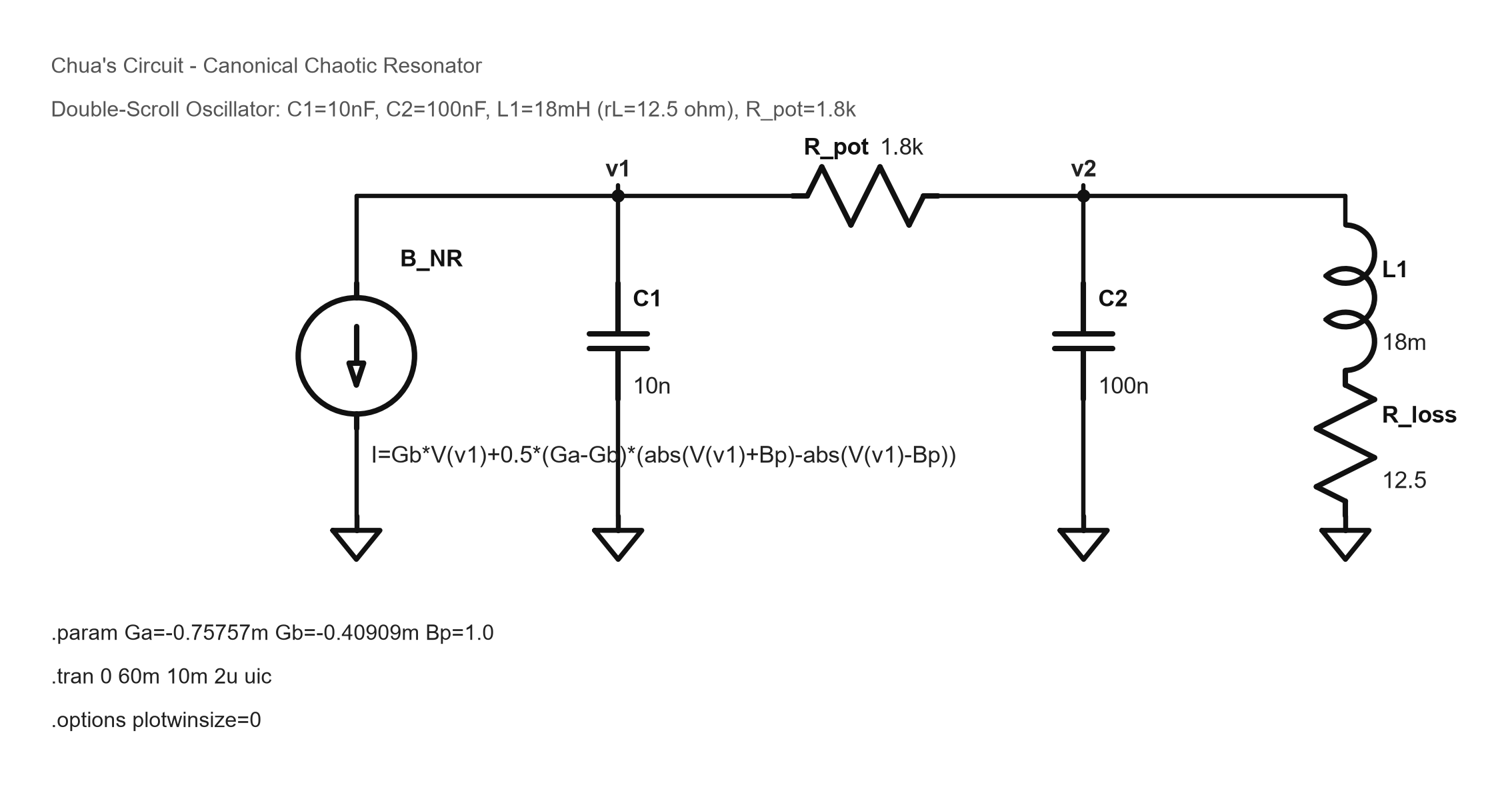
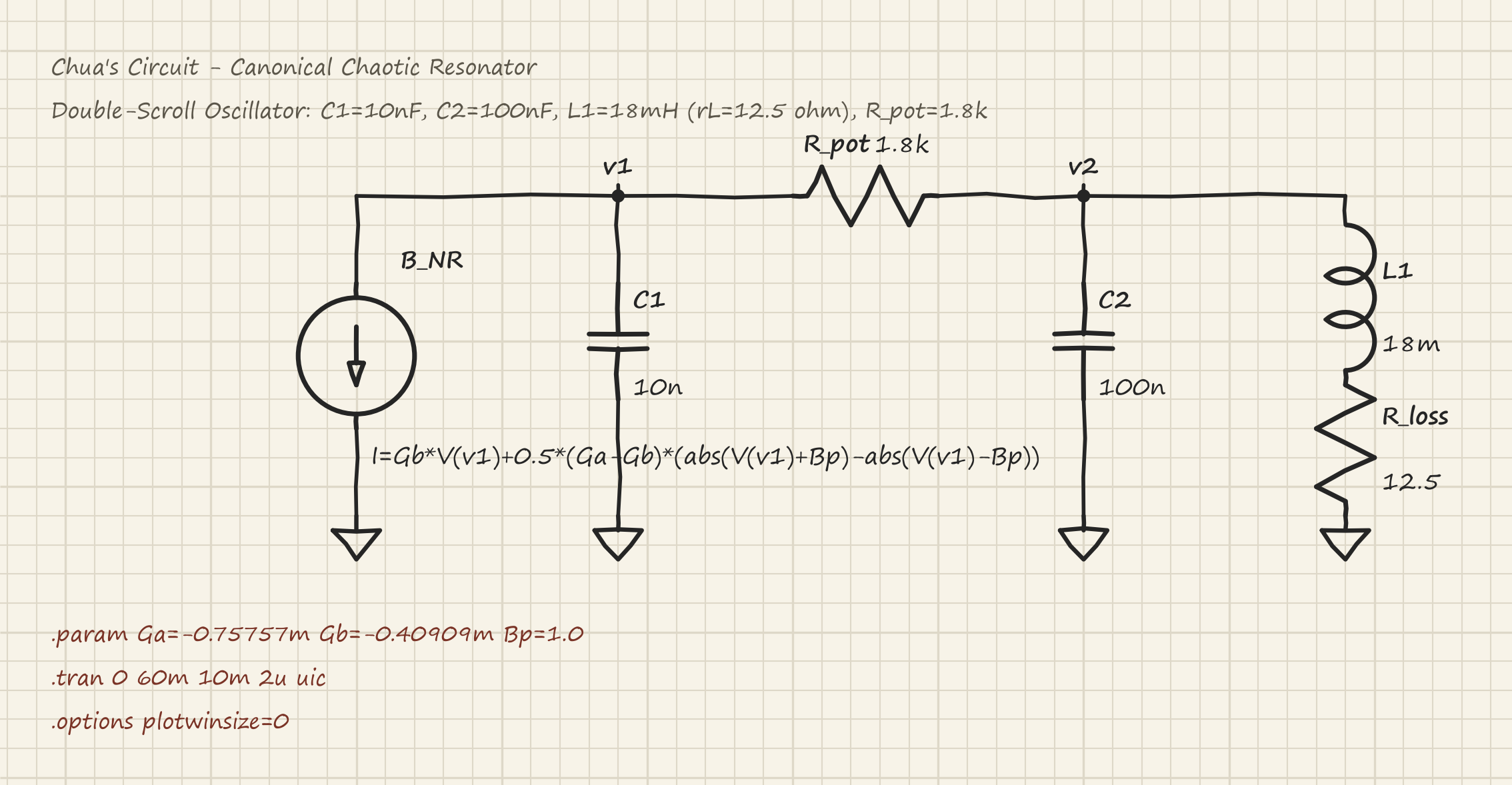
tech_minimal(default): charcoal ink, with colour reserved strictly for signal information like inputs, outputs, and feedback paths.classic: monochrome, engineered for crisp print and formal publication.sketch: engineering notebook style on graph paper with subtle hand drawn variation, while preserving exact circuit topology.
The canvas is computed from the schematic's own bounding box, so nothing is cropped and there is no
empty page. The same file and style produce identical bytes every time: sketch wobble is
hashed deterministically from the geometry rather than drawn from an RNG. Label collisions are automatically detected and avoided.
Visual style & colour palette
The MCP resource spicemcp://style exposes the exact design tokens and colour ramp used
across all schematic renders and waveform plots. Read this instead of guessing colours when
composing figures, documentation, or web interfaces that sit alongside SpiceMCP output.
It returns default_style, schematic_styles, series, series_roles, chrome, fonts.
Waveform plots (generate_design_report, spicemcp.plots) draw their traces from a unified
five colour data visualization ramp and their chrome from tech_minimal:
| role | token | default | usage |
|---|---|---|---|
| Primary trace | C_TRACE |
#1E56A0 |
Main response curves (gain, step output, THD fundamental) |
| Secondary trace & bars | C_TRACE2 |
#38A3A5 |
Phase curves, input signals, FFT harmonic bars |
| Measured points | C_MARK |
#D9534F |
Critical points such as −3 dB cutoff, overshoot peaks, and unity crossings |
| Limits & specifications | C_LIMIT |
#E07A5F |
Target thresholds, mask boundaries, upper/lower bounds |
| Margin bands & tolerance | C_BAND |
#F2CC8F |
Settling error bands (±1%, ±0.1%) and tolerance envelopes |
The series ramp is a monotonic lightness sweep that degrades cleanly in greyscale printing,
while maintaining maximum hue contrast between the first two traces for dual axis plots.
Sweeping a parameter
simulate with sweep_param and sweep_values runs one LTspice launch for the whole sweep via .step, and resolves the
parameter name against the deck so an ordinary netlist can be swept without being
reauthored as a template:
simulate(netlist, sweep_param="temp",   sweep_values=[-40, 27, 125])  # .step temp list
simulate(netlist, sweep_param="{GAIN}", sweep_values=[10, 20, 50])    # placeholder
simulate(netlist, sweep_param="R1",     sweep_values=[1e3, 2e3, 5e3]) # literal value
One row per point, and each row's value is read back from what LTspice itself reported
rather than from what was requested. A point the simulator skipped cannot shift the rest
of the table onto the wrong values. value_source indicates the source of evidence: the
log's .step echo, the .raw sweep axis (a stepped .op leaves no echo in the log, so the
axis is the sole record), or requested for a row nothing reported. A deck with no .meas
still returns its points and its raw_path, plus a warning explaining why the metrics are
empty.
The final design report
generate_design_report writes the entire report: six sections of Markdown where every number
is read out of state.db or out of a simulation launched while writing the file. Nothing is
hand entered, ensuring the report cannot disagree with the run it describes.
python -m spicemcp.report amp_001 --dc-audit --pvt --supply V1 --mc 100
# .ltspice-mcp/reports/amp_001_DESIGN_REPORT.md
generate_design_report(run_id="amp_001", dc_audit=True, pvt=True,
                       supply="V1", monte_carlo=100, schematic="pics/amp.png")
| section | contents |
|---|---|
| 1: Executive summary | topology and what the run establishes, constraint scorecard |
| 2: Schematic & BOM | designators, optimized values in engineering units (81.4 kΩ, 12.2 nF), tuning parameter mapping, tolerance, .model cards, link to the byte exact .cir |
| 3: Optimization & verification | Metric │ Target │ Baseline │ Final │ Δ │ Status, measured sensitivities with method, tradeoffs, bound warnings |
| 4: Waveform analysis | Bode (gain, phase, −3 dB, PM/GM), transient (rise, overshoot, ±1% and ±0.1% settling, slew), FFT/THD, with plots |
| 5: Robustness | per-device Vds/Vgs/Vth/current/region, PVT corners, Monte Carlo yield and Cpk |
| 6: Reproduction guide | open the .cir, the directives already in it, F9, Ctrl+L |
Sections 1, 2, 3, and 6 are free queries against stored state. The rest each cost LTspice launches,
so they are opt in: one shared rerun of the winner (which draws the plots and reports whether
fresh metrics still match stored ones), plus dc_audit (1 launch), pvt (5 launches), and monte_carlo
(1 stepped run rather than N separate launches).
A section that did not run states that clearly and specifies which argument produces it.
A reviewer reads a missing heading as "checked, nothing to report", so an unswept corner analysis prints as> **Not run.** … To include it: generate(con, run_id, pvt=True) rather than being omitted or filled with zeros.
The same principle applies when check_feasibility reports checks_skipped at the beginning of the pipeline.
Two additional cases where missing data is made explicit:
- Monte Carlo yield is evaluated against the run's own constraints. Without an interval for
a metric, the table is labelled as a spread andpassis reported accurately as unverified. - No schematic is automatically generated from netlists alone, because netlists lack coordinates.
Passschematic=with an image drawn usingspicemcp.ascand validated viaasc.check().
Tools Reference
11 tools, each with a two-line description, typed inputs, and sensible defaults. Every
answer ends with next_step (the call that most likely comes next), and every error carriesfix plus a correct example call, so even a small model can recover on its own.
| tool | purpose |
|---|---|
check_setup |
Show the LTspice path and project folder in use |
simulate |
One-off netlist run, or a one-launch sweep (sweep_param, sweep_values) |
check_feasibility |
Zero-sim check (static, template, physics) before spending simulations |
start_optimization |
Create a persistent run: params, goals, limits |
run_optimization |
Let the server run N iterations; returns one summary |
evaluate_candidate |
Simulate one exact parameter set, with dedup and scoring |
query_run |
Read stored state: what = status, best, pareto, history, candidates, candidate, netlist, compare, similar, sensitivity, explored, failed, trace, next, runs |
rollback_to_candidate |
Restore a byte exact past circuit and its metrics |
stop_optimization |
Stop a run, keeping all state |
generate_design_report |
Six section Markdown report with BOM, plots, DC/PVT/Monte Carlo |
render_schematic |
Render .asc to SVG/PNG using real .asy geometry in 3 styles |
Upgrading from 0.5: the 15 get_* / list_runs / select_next_experiment tools are nowquery_run(what=...); simulate_netlist and simulate_sweep are simulate;check_ltspice is check_setup; get_visual_style is the spicemcp://style resource.
Guarantees worth knowing
- A worse iteration cannot demote the incumbent.
best_candidateis aMAX(score)
query, wherescoreis a pure function of a candidate's metrics (using fixed reference
scales defined at run creation). Nothing is overwritten, preventing state corruption. - Modification never mutates. A changed parameter set creates a new candidate record (
cand_NNNN)
linked to itsparent_id, preserving the complete derivation tree. - Duplicates are never resimulated. Deduplication checks
sha256(design) + sha256(sim_config).
Evaluating the same circuit under different conditions constitutes a distinct experiment rather than a duplicate. rollback_to_candidaterestores stored bytes directly from disk, never a reconstruction.- Sensitivities are measured empirically. The
finite_differencemethod indicates direct
causal pairs differing in a single parameter;ols_marginalindicates correlational fits across multiple runs. - Every parameter is screened initially. Parameters without variance have zero measured
sensitivity and cannot be selected by exploitation alone. Unmeasured parameters take priority
over unexploited ones. For decade spaced discrete lists, steps move to adjacent entries rather than
using proportional spans. - The search is scale free, cycles coordinates, and refines step sizes dynamically.
Coordinate descent accounts for dimensional scaling (e.g. farads vs ohms) by normalizing against
parameter bounds, alternates across coordinates to avoid greedy fixation, and halves step sizes
when progress stagnates to converge within narrow tolerance bands. - Failures are classified and remembered. The engine records failure modes (
convergence_failure,structural_error,constraint_violation,numerical_instability) to prevent redundant exploration of invalid parameter regions.
Deliberate simplifications
| skipped | add when |
|---|---|
scoring a candidate off a waveform (raw.py parses .raw, but objectives are .meas) |
a metric genuinely cannot be expressed as .meas (requires wave to scalar processing) |
| Bayesian optimization / GP surrogate | a single sim is fast enough that ~30 evaluations is cheaper than surrogate model complexity |
| step halving on stagnation instead of line search | evaluations spent bracketing cost more than simple step halving bookkeeping |
| one parameter moves per iteration (coordinate descent) | metric surface has strong parameter interactions requiring full compass polling |
| component graph IR (topology edits are new templates) | programmatic topology rewriting is explicitly required |
| incremental sensitivity updates (O(n²) per iteration) | runs exceed several hundred candidates |
promising_unexplored_region identifies the widest untried gap |
directional search hints are needed (the main search already uses measured sensitivity) |
asc.Sheet places parts at specified coordinates |
automated placement solver is available |
| the design report embeds user supplied schematics without auto layout | schematic autoplacer exists to render and validate netlists |
| report plot generation resimulates the winner | full waveform history is required for every intermediate candidate |
| preflight metric recognition uses standardized naming conventions | metric name collisions require explicit type annotations |
check_feasibility inspects top level netlist elements |
subcircuit internal pole modeling is required (handled during simulation in robustness) |
| W/L aspect ratio check requires explicit W and L parameters | device geometry is defined via unified size parameters or model cards |
render_schematic applies single pass greedy label collision offsets |
complex placement solver is required for high density schematics |
renderer draws explicitly defined .asc geometry without automatic placement |
layout synthesis engine is added |
simulate_sweep steps one parameter per launch |
nested 2D parameter sweeps are needed (run sequentially across outer values) |
Schematic rendering styles
render_schematic renders any .asc file into three distinct visual styles over identical circuit geometry:
Classic (classic) |
Sketch (sketch) |
Tech Minimal (tech_minimal) |
|---|---|---|
 |
 |
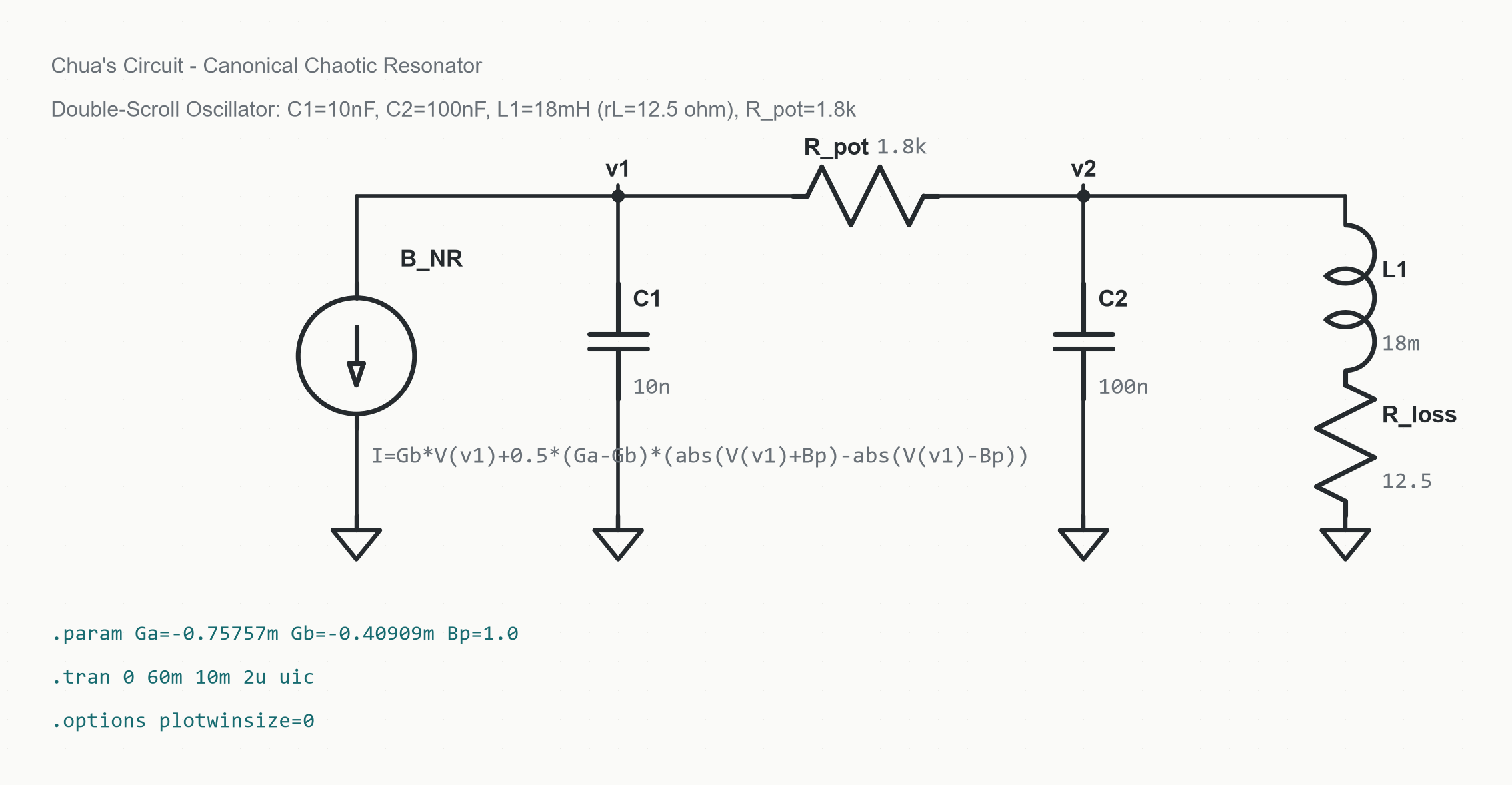 |
| Monochrome, high-contrast formal print style | Engineering notebook style on graph paper with deterministic hand-drawn wobble | Charcoal ink with semantic signal line and port highlighting |
Test suites & verification
- Hallucination Loop Test (
tests/test_hallucination_loop.py): drives the adversarial sequence (improve, improve, best, worse, worse, improve) and verifies the incumbent survives, candidate identities remain immutable, duplicates are rejected without simulation, and sensitivities match analytical derivatives. - Visual Gallery (
tests/gallery.py): renders side by side comparison sheets of every schematic style and plot type intogallery/index.htmlusing real.asylibrary symbols. - Preflight & Report Testing (
tests/test_feasibility.py,tests/test_report.py,tests/test_robustness.py): validates 3 tier feasibility checks, Monte Carlo yield and Cpk calculations, DC bias audits, and full Markdown report generation. - Rendering & Sweeps (
tests/test_render.py,tests/test_sweep.py,tests/test_asc.py): tests deterministic SVG and PNG rendering, symbol orientation matrices, collision offsets, and single launch parameter sweeps.
Yorumlar (0)
Yorum birakmak icin giris yap.
Yorum birakSonuc bulunamadi